確率キュー位置モデル
概要
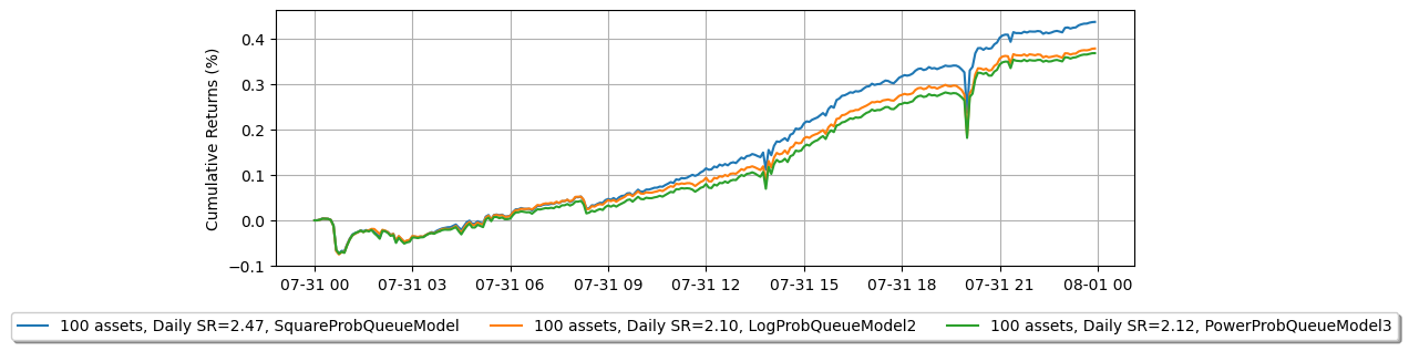
ここでは、キュー位置モデルが注文の充足シミュレーションにどのように影響し、最終的に戦略のパフォーマンスにどのように影響するかを示します。正確なバックテストを行うためには、バックテストと実際の取引結果を比較して適切なキュー位置モデルを見つけることが重要です。この文脈では、キュー位置モデルを変更することで比較を示します。これにより、バックテストと実際の取引結果が一致する適切なキュー位置モデルを特定できます。
注: この例は教育目的のみであり、高頻度マーケットメイキングスキームの効果的な戦略を示しています。すべてのバックテストは、Binance Futuresで利用可能な最高のマーケットメイカーリベートである0.005%のリベートに基づいています。詳細については、Binance Upgrades USDⓢ-Margined Futures Liquidity Provider Program を参照してください。
[1]:
import numpy as np

from numba import njit, uint64
from numba.typed import Dict

from hftbacktest import (
    BacktestAsset,
    ROIVectorMarketDepthBacktest,
    GTX,
    LIMIT,
    BUY,
    SELL,
    BUY_EVENT,
    SELL_EVENT,
    Recorder
)
from hftbacktest.stats import LinearAssetRecord

@njit(cache=True)
def measure_trading_intensity(order_arrival_depth, out):
    max_tick = 0
    for depth in order_arrival_depth:
        if not np.isfinite(depth):
            continue

        # Sets the tick index to 0 for the nearest possible best price
        # as the order arrival depth in ticks is measured from the mid-price
        tick = round(depth / .5) - 1

        # In a fast-moving market, buy trades can occur below the mid-price (and vice versa for sell trades)
        # since the mid-price is measured in a previous time-step;
        # however, to simplify the problem, we will exclude those cases.
        if tick < 0 or tick >= len(out):
            continue

        # All of our possible quotes within the order arrival depth,
        # excluding those at the same price, are considered executed.
        out[:tick] += 1

        max_tick = max(max_tick, tick)
    return out[:max_tick]

@njit(cache=True)
def linear_regression(x, y):
    sx = np.sum(x)
    sy = np.sum(y)
    sx2 = np.sum(x ** 2)
    sxy = np.sum(x * y)
    w = len(x)
    slope = (w * sxy - sx * sy) / (w * sx2 - sx**2)
    intercept = (sy - slope * sx) / w
    return slope, intercept

@njit(cache=True)
def compute_coeff_simplified(gamma, delta, A, k):
    inv_k = np.divide(1, k)
    c1 = inv_k
    c2 = np.sqrt(np.divide(gamma * np.exp(1), 2 * A * delta * k))
    return c1, c2

@njit
def gridtrading_glft_mm(hbt, recorder, gamma, order_qty):
    asset_no = 0
    tick_size = hbt.depth(asset_no).tick_size

    arrival_depth = np.full(30_000_000, np.nan, np.float64)
    mid_price_chg = np.full(30_000_000, np.nan, np.float64)

    t = 0
    prev_mid_price_tick = np.nan
    mid_price_tick = np.nan

    tmp = np.zeros(500, np.float64)
    ticks = np.arange(len(tmp)) + 0.5

    A = np.nan
    k = np.nan
    volatility = np.nan
    delta = 1

    grid_num = 20
    max_position = 50 * order_qty

    # Checks every 100 milliseconds.
    while hbt.elapse(100_000_000) == 0:
        #--------------------------------------------------------
        # Records market order's arrival depth from the mid-price.
        if not np.isnan(mid_price_tick):
            depth = -np.inf
            for last_trade in hbt.last_trades(asset_no):
                trade_price_tick = last_trade.px / tick_size

                if last_trade.ev & BUY_EVENT == BUY_EVENT:
                    depth = max(trade_price_tick - mid_price_tick, depth)
                else:
                    depth = max(mid_price_tick - trade_price_tick, depth)
            arrival_depth[t] = depth

        hbt.clear_last_trades(asset_no)
        hbt.clear_inactive_orders(asset_no)

        depth = hbt.depth(asset_no)
        position = hbt.position(asset_no)
        orders = hbt.orders(asset_no)

        best_bid_tick = depth.best_bid_tick
        best_ask_tick = depth.best_ask_tick

        prev_mid_price_tick = mid_price_tick
        mid_price_tick = (best_bid_tick + best_ask_tick) / 2.0

        # Records the mid-price change for volatility calculation.
        mid_price_chg[t] = mid_price_tick - prev_mid_price_tick

        #--------------------------------------------------------
        # Calibrates A, k and calculates the market volatility.

        # Updates A, k, and the volatility every 5-sec.
        if t % 50 == 0:
            # Window size is 10-minute.
            if t >= 6_000 - 1:
                # Calibrates A, k
                tmp[:] = 0
                lambda_ = measure_trading_intensity(arrival_depth[t + 1 - 6_000:t + 1], tmp)
                if len(lambda_) > 2:
                    lambda_ = lambda_[:70] / 600
                    x = ticks[:len(lambda_)]
                    y = np.log(lambda_)
                    k_, logA = linear_regression(x, y)
                    A = np.exp(logA)
                    k = -k_

                # Updates the volatility.
                volatility = np.nanstd(mid_price_chg[t + 1 - 6_000:t + 1]) * np.sqrt(10)

        #--------------------------------------------------------
        # Computes bid price and ask price.

        c1, c2 = compute_coeff_simplified(gamma, delta, A, k)

        half_spread_tick = c1 + delta / 2 * c2 * volatility
        skew = c2 * volatility

        normalized_position = position / order_qty

        reservation_price_tick = mid_price_tick - skew * normalized_position

        bid_price_tick = min(np.round(reservation_price_tick - half_spread_tick), best_bid_tick)
        ask_price_tick = max(np.round(reservation_price_tick + half_spread_tick), best_ask_tick)

        bid_price = bid_price_tick * tick_size
        ask_price = ask_price_tick * tick_size

        grid_interval = max(np.round(half_spread_tick) * tick_size, tick_size)

        bid_price = np.floor(bid_price / grid_interval) * grid_interval
        ask_price = np.ceil(ask_price / grid_interval) * grid_interval

        #--------------------------------------------------------
        # Updates quotes.

        # Creates a new grid for buy orders.
        new_bid_orders = Dict.empty(np.uint64, np.float64)
        if position < max_position and np.isfinite(bid_price):
            for i in range(grid_num):
                bid_price_tick = round(bid_price / tick_size)

                # order price in tick is used as order id.
                new_bid_orders[uint64(bid_price_tick)] = bid_price

                bid_price -= grid_interval

        # Creates a new grid for sell orders.
        new_ask_orders = Dict.empty(np.uint64, np.float64)
        if position > -max_position and np.isfinite(ask_price):
            for i in range(grid_num):
                ask_price_tick = round(ask_price / tick_size)

                # order price in tick is used as order id.
                new_ask_orders[uint64(ask_price_tick)] = ask_price

                ask_price += grid_interval

        order_values = orders.values();
        while order_values.has_next():
            order = order_values.get()
            # Cancels if a working order is not in the new grid.
            if order.cancellable:
                if (
                    (order.side == BUY and order.order_id not in new_bid_orders)
                    or (order.side == SELL and order.order_id not in new_ask_orders)
                ):
                    hbt.cancel(asset_no, order.order_id, False)

        for order_id, order_price in new_bid_orders.items():
            # Posts a new buy order if there is no working order at the price on the new grid.
            if order_id not in orders:
                hbt.submit_buy_order(asset_no, order_id, order_price, order_qty, GTX, LIMIT, False)

        for order_id, order_price in new_ask_orders.items():
            # Posts a new sell order if there is no working order at the price on the new grid.
            if order_id not in orders:
                hbt.submit_sell_order(asset_no, order_id, order_price, order_qty, GTX, LIMIT, False)

        #--------------------------------------------------------
        # Records variables and stats for analysis.

        t += 1

        if t >= len(arrival_depth) or t >= len(mid_price_chg):
            raise Exception

        # Records the current state for stat calculation.
        recorder.record(hbt)
[2]:
def backtest(args):
    asset_name, asset_info, model = args

    # Obtains the mid-price of the assset to determine the order quantity.
    snapshot = np.load('data/{}_20230730_eod.npz'.format(asset_name))['data']
    best_bid = max(snapshot[snapshot['ev'] & BUY_EVENT == BUY_EVENT]['px'])
    best_ask = min(snapshot[snapshot['ev'] & SELL_EVENT == SELL_EVENT]['px'])
    mid_price = (best_bid + best_ask) / 2.0

    latency_data = np.concatenate(
        [np.load('latency/live_order_latency_{}.npz'.format(date))['data'] for date in range(20230731, 20230732)]
    )

    asset = (
        BacktestAsset()
            .data(['data/{}_{}.npz'.format(asset_name, date) for date in range(20230731, 20230732)])
            .initial_snapshot('data/{}_20230730_eod.npz'.format(asset_name))
            .linear_asset(1.0)
            .intp_order_latency(latency_data)
            .no_partial_fill_exchange()
            .trading_value_fee_model(-0.00005, 0.0007)
            .tick_size(asset_info['tick_size'])
            .lot_size(asset_info['lot_size'])
            .roi_lb(0.0)
            .roi_ub(mid_price * 5)
            .last_trades_capacity(10000)
    )

    if model == 'SquareProbQueueModel':
        asset.power_prob_queue_model(2)
    elif model == 'LogProbQueueModel2':
        asset.log_prob_queue_model2()
    elif model == 'PowerProbQueueModel3':
        asset.power_prob_queue_model3(3)
    else:
        raise ValueError


    hbt = ROIVectorMarketDepthBacktest([asset])

    # Sets the order quantity to be equivalent to a notional value of $100.
    order_qty = max(round((100 / mid_price) / asset_info['lot_size']), 1) * asset_info['lot_size']

    recorder = Recorder(1, 30_000_000)

    gamma = 0.00005
    gridtrading_glft_mm(hbt, recorder.recorder, gamma, order_qty)

    hbt.close()

    recorder.to_npz('stats/gridtrading_simple_glft_qm_{}_{}.npz'.format(model, asset_name))
[3]:
%%capture
from multiprocessing import Pool
import json

with open('assets2.json', 'r') as f:
    assets = json.load(f)

with Pool(16) as p:
    print(p.map(backtest, [(k, v, 'SquareProbQueueModel') for k, v in assets.items()]))

with Pool(16) as p:
    print(p.map(backtest, [(k, v, 'LogProbQueueModel2') for k, v in assets.items()]))

with Pool(16) as p:
    print(p.map(backtest, [(k, v, 'PowerProbQueueModel3') for k, v in assets.items()]))
[4]:
import polars as pl
from matplotlib import pyplot as plt

def compute_net_equity(model):
    equity_values = {}
    sr_values = {}

    for asset_name in assets.keys():
        data = np.load('stats/gridtrading_simple_glft_qm_{}_{}.npz'.format(model, asset_name))['0']
        stats = (
            LinearAssetRecord(data)
                .resample('5m')
                .stats()
        )

        equity = stats.entire.with_columns(
            (pl.col('equity_wo_fee') - pl.col('fee')).alias('equity')
        ).select(['timestamp', 'equity'])

        pnl = equity['equity'].diff()
        sr = np.divide(pnl.mean(), pnl.std())

        equity_values[asset_name] = equity
        sr_values[asset_name] = sr

    sr_m = np.nanmean(list(sr_values.values()))
    sr_s = np.nanstd(list(sr_values.values()))

    asset_number = 0
    net_equity = None
    for i, (equity, sr) in enumerate(zip(equity_values.values(), sr_values.values())):
        # There are some assets that aren't working within this scheme.
        # This might be because the order arrivals don't follow a Poisson distribution that this model assumes.
        # As a result, it filters out assets whose SR falls outside -0.5 sigma.
        if (sr - sr_m) / sr_s > -0.5:
            asset_number += 1
            if net_equity is None:
                net_equity = equity.clone()
            else:
                net_equity = net_equity.select(
                    'timestamp',
                    (pl.col('equity') + equity['equity']).alias('equity')
                )

            if asset_number == 100:
                # 5_000 is capital for each trading asset.
                return net_equity.with_columns(
                    (pl.col('equity') / asset_number / 5_000).alias('equity')
                )

np.seterr(divide='ignore', invalid='ignore')

fig = plt.figure()
fig.set_size_inches(10, 3)
legend = []

for model in ['SquareProbQueueModel', 'LogProbQueueModel2', 'PowerProbQueueModel3']:
    net_equity_ = compute_net_equity(model)

    pnl = net_equity_['equity'].diff()
    # Since the P&L is resampled at a 5-minute interval
    sr = pnl.mean() / pnl.std() * np.sqrt(24 * 60 / 5)
    legend.append('100 assets, Daily SR={:.2f}, {}'.format(sr, model))
    plt.plot(net_equity_['timestamp'], net_equity_['equity'] * 100)

plt.legend(
    legend,
    loc='upper center', bbox_to_anchor=(0.5, -0.15),
    fancybox=True, shadow=True, ncol=3
)

plt.grid()
plt.ylabel('Cumulative Returns (%)')
[4]:
Text(0, 0.5, 'Cumulative Returns (%)')