複数の市場を作る
概要
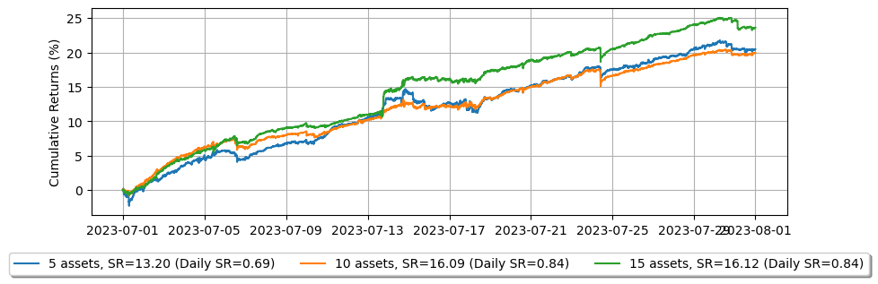
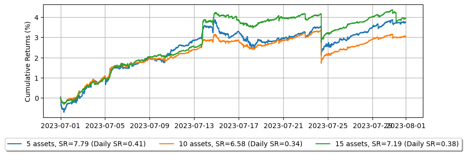
資産を分散し、市場作りのブックを構築することで、分散効果を通じてリスク調整後のリターンを向上させることができます。この例では、市場を作る資産の数を増やすにつれて、市場作りポートフォリオの統計がどのように変化するかを示します。
GLFTマーケットメイキングモデルを使用して複数の資産でグリッドトレーディングを実装するには、いくつかの修正が必要です。パラメータを調整する必要はありません。
資産ごとに価格、取引量、オーダーブックの流動性が異なるため、注文数量が異なります。すべてを一度にバックテストするには、注文数量を正規化し、それに応じて調整する必要があります。
一部の資産では、市場取引が主に最良買い気配値と最良売り気配値のレベルで行われます。市場取引が私たちのクォートと一致する場合にのみ取引強度を計算するため、そのような場合には取引強度関数に適した取引強度を達成できない可能性があります。その結果、オーダー到着深度に基づいてハーフスプレッドとスキューを決定するための代替方法を検討する必要があります。または、より深いオーダー到着深度を得るために反応間隔を増やす必要がありますが、これは特に急速に動く市場では遅延反応を引き起こします。
\(adj_2\)が異なる注文数量を正規化するためにどのように決定されるかを確認してください。
注: この例は教育目的のみであり、高頻度マーケットメイキングスキームの効果的な戦略を示しています。すべてのバックテストは、Binance Futuresで利用可能な最高のマーケットメイカーリベートである0.005%のリベートに基づいています。詳細については、Binance Upgrades USDⓢ-Margined Futures Liquidity Provider Program を参照してください。
[1]:
import numpy as np

from numba import njit, uint64
from numba.typed import Dict

from hftbacktest import (
    BacktestAsset,
    ROIVectorMarketDepthBacktest,
    GTX,
    LIMIT,
    BUY,
    SELL,
    BUY_EVENT,
    SELL_EVENT,
    Recorder
)
from hftbacktest.stats import LinearAssetRecord


@njit(cache=True)
def measure_trading_intensity(order_arrival_depth, out):
    max_tick = 0
    for depth in order_arrival_depth:
        if not np.isfinite(depth):
            continue

        # Sets the tick index to 0 for the nearest possible best price
        # as the order arrival depth in ticks is measured from the mid-price
        tick = round(depth / .5) - 1

        # In a fast-moving market, buy trades can occur below the mid-price (and vice versa for sell trades)
        # since the mid-price is measured in a previous time-step;
        # however, to simplify the problem, we will exclude those cases.
        if tick < 0 or tick >= len(out):
            continue

        # All of our possible quotes within the order arrival depth,
        # excluding those at the same price, are considered executed.
        out[:tick] += 1

        max_tick = max(max_tick, tick)
    return out[:max_tick]


@njit(cache=True)
def compute_coeff(xi, gamma, delta, A, k):
    inv_k = np.divide(1, k)
    c1 = 1 / (xi * delta) * np.log(1 + xi * delta * inv_k)
    c2 = np.sqrt(np.divide(gamma, 2 * A * delta * k) * ((1 + xi * delta * inv_k) ** (k / (xi * delta) + 1)))
    return c1, c2


@njit(cache=True)
def linear_regression(x, y):
    sx = np.sum(x)
    sy = np.sum(y)
    sx2 = np.sum(x ** 2)
    sxy = np.sum(x * y)
    w = len(x)
    slope = np.divide(w * sxy - sx * sy, w * sx2 - sx**2)
    intercept = np.divide(sy - slope * sx, w)
    return slope, intercept


@njit
def gridtrading_glft_mm(hbt, recorder, order_qty):
    asset_no = 0
    tick_size = hbt.depth(asset_no).tick_size

    arrival_depth = np.full(30_000_000, np.nan, np.float64)
    mid_price_chg = np.full(30_000_000, np.nan, np.float64)

    t = 0
    prev_mid_price_tick = np.nan
    mid_price_tick = np.nan

    tmp = np.zeros(500, np.float64)
    ticks = np.arange(len(tmp)) + 0.5

    A = np.nan
    k = np.nan
    volatility = np.nan
    gamma = 0.05
    delta = 1
    adj1 = 1

    # adj2 is determined according to the order quantity.
    grid_num = 20
    max_position = grid_num * order_qty
    adj2 = 1 / max_position

    # Checks every 100 milliseconds.
    while hbt.elapse(100_000_000) == 0:
        #--------------------------------------------------------
        # Records market order's arrival depth from the mid-price.
        if not np.isnan(mid_price_tick):
            depth = -np.inf
            for last_trade in hbt.last_trades(asset_no):
                trade_price_tick = last_trade.px / tick_size

                if last_trade.ev & BUY_EVENT == BUY_EVENT:
                    depth = max(trade_price_tick - mid_price_tick, depth)
                else:
                    depth = max(mid_price_tick - trade_price_tick, depth)
            arrival_depth[t] = depth

        hbt.clear_last_trades(asset_no)
        hbt.clear_inactive_orders(asset_no)

        depth = hbt.depth(asset_no)
        position = hbt.position(asset_no)
        orders = hbt.orders(asset_no)

        best_bid_tick = depth.best_bid_tick
        best_ask_tick = depth.best_ask_tick

        prev_mid_price_tick = mid_price_tick
        mid_price_tick = (best_bid_tick + best_ask_tick) / 2.0

        # Records the mid-price change for volatility calculation.
        mid_price_chg[t] = mid_price_tick - prev_mid_price_tick

        #--------------------------------------------------------
        # Calibrates A, k and calculates the market volatility.

        # Updates A, k, and the volatility every 5-sec.
        if t % 50 == 0:
            # Window size is 10-minute.
            if t >= 6_000 - 1:
                # Calibrates A, k
                tmp[:] = 0
                lambda_ = measure_trading_intensity(arrival_depth[t + 1 - 6_000:t + 1], tmp)
                if len(lambda_) > 2:
                    lambda_ = lambda_[:70] / 600
                    x = ticks[:len(lambda_)]
                    y = np.log(lambda_)
                    k_, logA = linear_regression(x, y)
                    A = np.exp(logA)
                    k = -k_

                # Updates the volatility.
                volatility = np.nanstd(mid_price_chg[t + 1 - 6_000:t + 1]) * np.sqrt(10)

        #--------------------------------------------------------
        # Computes bid price and ask price.

        c1, c2 = compute_coeff(gamma, gamma, delta, A, k)

        half_spread_tick = (c1 + delta / 2 * c2 * volatility) * adj1
        skew = c2 * volatility * adj2

        reservation_price_tick = mid_price_tick - skew * position

        bid_price_tick = min(np.round(reservation_price_tick - half_spread_tick), best_bid_tick)
        ask_price_tick = max(np.round(reservation_price_tick + half_spread_tick), best_ask_tick)

        bid_price = bid_price_tick * tick_size
        ask_price = ask_price_tick * tick_size

        grid_interval = max(np.round(half_spread_tick) * tick_size, tick_size)

        bid_price = np.floor(bid_price / grid_interval) * grid_interval
        ask_price = np.ceil(ask_price / grid_interval) * grid_interval

        #--------------------------------------------------------
        # Updates quotes.

        # Creates a new grid for buy orders.
        new_bid_orders = Dict.empty(np.uint64, np.float64)
        if position < max_position and np.isfinite(bid_price):
            for i in range(grid_num):
                bid_price_tick = round(bid_price / tick_size)

                # order price in tick is used as order id.
                new_bid_orders[uint64(bid_price_tick)] = bid_price

                bid_price -= grid_interval

        # Creates a new grid for sell orders.
        new_ask_orders = Dict.empty(np.uint64, np.float64)
        if position > -max_position and np.isfinite(ask_price):
            for i in range(grid_num):
                ask_price_tick = round(ask_price / tick_size)

                # order price in tick is used as order id.
                new_ask_orders[uint64(ask_price_tick)] = ask_price

                ask_price += grid_interval

        order_values = orders.values();
        while order_values.has_next():
            order = order_values.get()
            # Cancels if a working order is not in the new grid.
            if order.cancellable:
                if (
                    (order.side == BUY and order.order_id not in new_bid_orders)
                    or (order.side == SELL and order.order_id not in new_ask_orders)
                ):
                    hbt.cancel(asset_no, order.order_id, False)

        for order_id, order_price in new_bid_orders.items():
            # Posts a new buy order if there is no working order at the price on the new grid.
            if order_id not in orders:
                hbt.submit_buy_order(asset_no, order_id, order_price, order_qty, GTX, LIMIT, False)

        for order_id, order_price in new_ask_orders.items():
            # Posts a new sell order if there is no working order at the price on the new grid.
            if order_id not in orders:
                hbt.submit_sell_order(asset_no, order_id, order_price, order_qty, GTX, LIMIT, False)

        #--------------------------------------------------------
        # Records variables and stats for analysis.

        t += 1

        if t >= len(arrival_depth) or t >= len(mid_price_chg):
            raise Exception

        # Records the current state for stat calculation.
        recorder.record(hbt)
注文数量は、$100の名目価値に相当するように決定されます。
[2]:
def backtest(args):
    asset_name, asset_info = args

    # Obtains the mid-price of the assset to determine the order quantity.
    snapshot = np.load('data/{}_20230630_eod.npz'.format(asset_name))['data']
    best_bid = max(snapshot[snapshot['ev'] & BUY_EVENT == BUY_EVENT]['px'])
    best_ask = min(snapshot[snapshot['ev'] & SELL_EVENT == SELL_EVENT]['px'])
    mid_price = (best_bid + best_ask) / 2.0

    latency_data = np.concatenate(
        [np.load('latency/feed_latency_{}.npz'.format(date))['data'] for date in range(20230701, 20230732)]
    )

    asset = (
        BacktestAsset()
            .data(['data/{}_{}.npz'.format(asset_name, date) for date in range(20230701, 20230732)])
            .initial_snapshot('data/{}_20230630_eod.npz'.format(asset_name))
            .linear_asset(1.0)
            .intp_order_latency(latency_data)
            .power_prob_queue_model(2.0)
            .no_partial_fill_exchange()
            .trading_value_fee_model(-0.00005, 0.0007)
            .tick_size(asset_info['tick_size'])
            .lot_size(asset_info['lot_size'])
            .roi_lb(0.0)
            .roi_ub(mid_price * 5)
            .last_trades_capacity(10000)
    )

    hbt = ROIVectorMarketDepthBacktest([asset])

    # Sets the order quantity to be equivalent to a notional value of $100.
    order_qty = max(round((100 / mid_price) / asset_info['lot_size']), 1) * asset_info['lot_size']

    recorder = Recorder(1, 30_000_000)

    gridtrading_glft_mm(hbt, recorder.recorder, order_qty)

    hbt.close()

    recorder.to_npz('stats/gridtrading_glft_mm_{}.npz'.format(asset_name))
マルチプロセッシングを利用することで、複数の資産のバックテストを同時に実行できます。
[3]:
%%capture
import json

from multiprocessing import Pool

with open('assets.json', 'r') as f:
    assets = json.load(f)

with Pool(16) as p:
    print(p.map(backtest, list(assets.items())))
[4]:
import polars as pl
from hftbacktest.stats import LinearAssetRecord

equity_values = {}
for asset_name in assets.keys():
    data = np.load('stats/gridtrading_glft_mm_{}.npz'.format(asset_name))['0']
    stats = (
        LinearAssetRecord(data)
            .resample('5m')
            .stats()
    )

    equity = stats.entire.with_columns(
        (pl.col('equity_wo_fee') - pl.col('fee')).alias('equity')
    ).select(['timestamp', 'equity'])
    equity_values[asset_name] = equity
個々の資産のエクイティカーブを確認し、複数の資産を組み合わせることで、エクイティカーブがより滑らかになり、リスク調整後のリターンが向上することに気付くことができます。
[5]:
from matplotlib import pyplot as plt

for i, asset_name in enumerate(assets.keys()):
    plt.figure(i, figsize=(10, 3))
    plt.plot(equity_values[asset_name]['timestamp'], equity_values[asset_name]['equity'])
    plt.grid()
    plt.title(asset_name)
    plt.ylabel('Equity ($)')
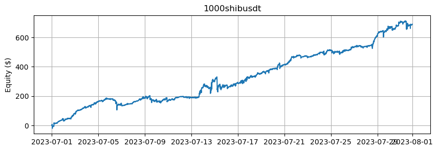
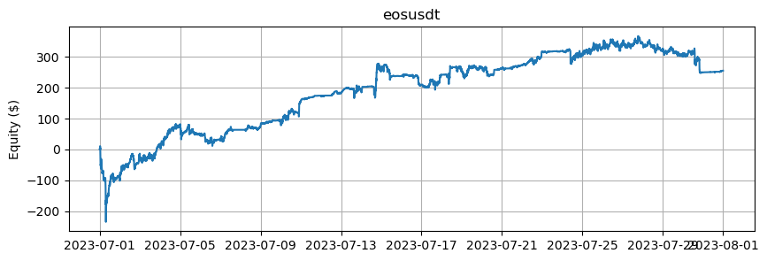
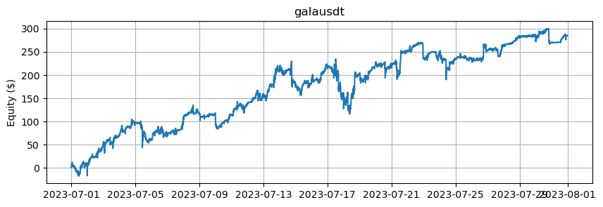
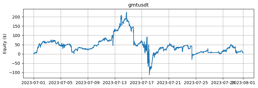
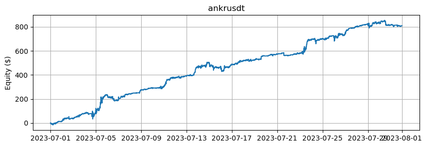
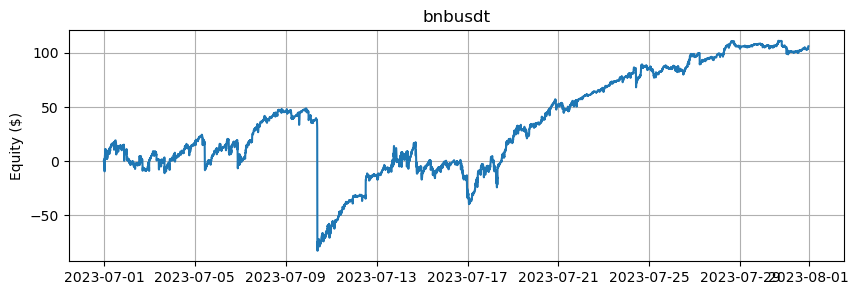
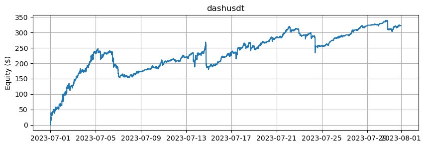
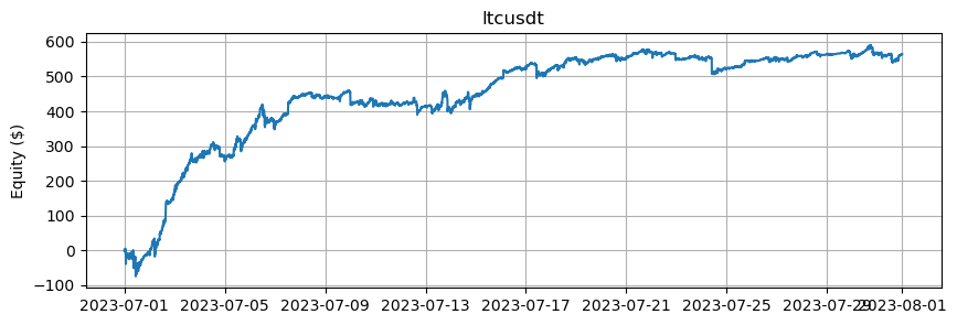
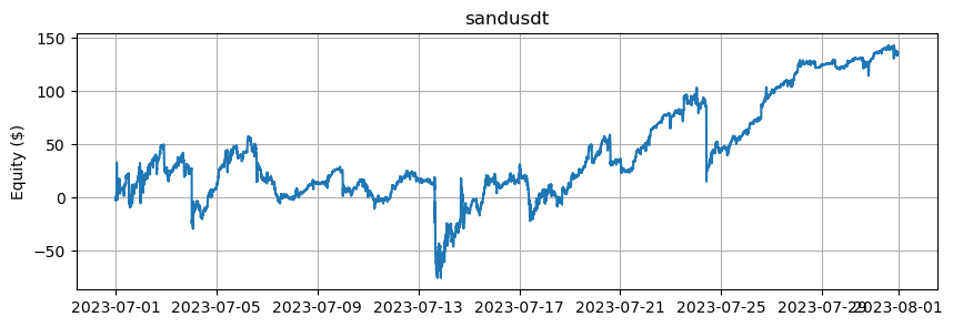
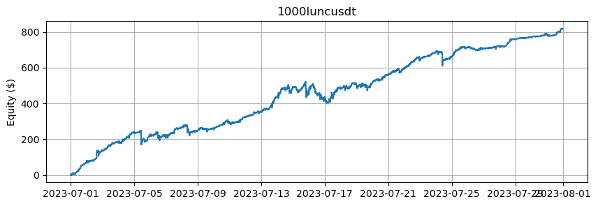
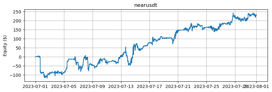
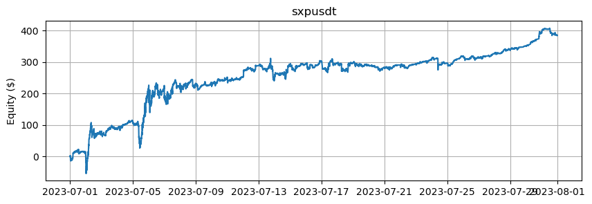
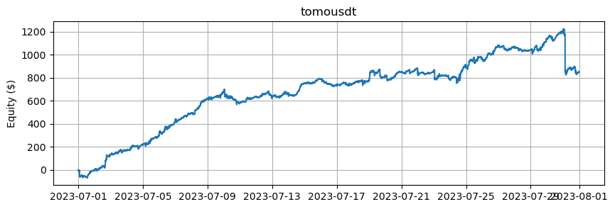
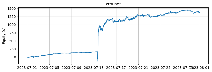
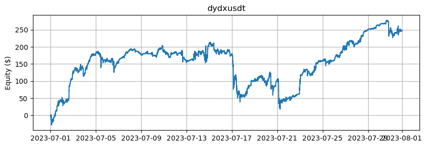
これは、BTCとETHを除くアルトコインの数に基づいたエクイティカーブを示しています。
[6]:
from matplotlib import pyplot as plt

fig = plt.figure()
fig.set_size_inches(10, 3)

legend = []
net_equity = None
for i, equity in enumerate(list(equity_values.values())):
    asset_number = i + 1
    if net_equity is None:
        net_equity = equity['equity'].clone()
    else:
        net_equity += equity['equity'].clone()

    if asset_number % 5 == 0:
        # 2_000 is capital for each trading asset.
        net_equity_df = pl.DataFrame({
            'cum_ret': (net_equity / asset_number) / 2_000 * 100,
            'timestamp': equity['timestamp']
        })
        net_equity_rs_df = net_equity_df.group_by_dynamic(
            index_column='timestamp',
            every='1d'
        ).agg([
            pl.col('cum_ret').last()
        ])
        pnl = net_equity_rs_df['cum_ret'].diff()
        sr = pnl.mean() / pnl.std()
        ann_sr = sr * np.sqrt(365)

        plt.plot(net_equity_df['timestamp'], net_equity_df['cum_ret'])
        legend.append('{} assets, SR={:.2f} (Daily SR={:.2f})'.format(asset_number, ann_sr, sr))

plt.legend(
    legend,
    loc='upper center', bbox_to_anchor=(0.5, -0.15),
    fancybox=True, shadow=True, ncol=3
)

plt.grid()
plt.ylabel('Cumulative Returns (%)')
[6]:
Text(0, 0.5, 'Cumulative Returns (%)')
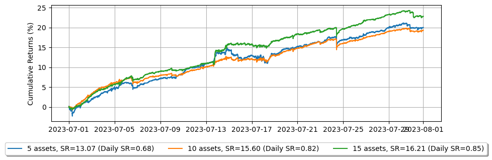
注文遅延の影響
増幅されたフィードレイテンシを適用すると、レイテンシの影響によりパフォーマンスが低下することがわかります。
[7]:
def backtest(args):
    asset_name, asset_info = args

    # Obtains the mid-price of the assset to determine the order quantity.
    snapshot = np.load('data/{}_20230630_eod.npz'.format(asset_name))['data']
    best_bid = max(snapshot[snapshot['ev'] & BUY_EVENT == BUY_EVENT]['px'])
    best_ask = min(snapshot[snapshot['ev'] & SELL_EVENT == SELL_EVENT]['px'])
    mid_price = (best_bid + best_ask) / 2.0

    latency_data = np.concatenate(
        [np.load('latency/amp_feed_latency_{}.npz'.format(date))['data'] for date in range(20230701, 20230732)]
    )

    asset = (
        BacktestAsset()
            .data(['data/{}_{}.npz'.format(asset_name, date) for date in range(20230701, 20230732)])
            .initial_snapshot('data/{}_20230630_eod.npz'.format(asset_name))
            .linear_asset(1.0)
            .intp_order_latency(latency_data)
            .power_prob_queue_model(2.0)
            .no_partial_fill_exchange()
            .trading_value_fee_model(-0.00005, 0.0007)
            .tick_size(asset_info['tick_size'])
            .lot_size(asset_info['lot_size'])
            .roi_lb(0.0)
            .roi_ub(mid_price * 5)
            .last_trades_capacity(10000)
    )

    hbt = ROIVectorMarketDepthBacktest([asset])

    # Sets the order quantity to be equivalent to a notional value of $100.
    order_qty = max(round((100 / mid_price) / asset_info['lot_size']), 1) * asset_info['lot_size']

    recorder = Recorder(1, 30_000_000)

    gridtrading_glft_mm(hbt, recorder.recorder, order_qty)

    hbt.close()

    recorder.to_npz('stats/gridtrading_glft_mm_lat1_{}.npz'.format(asset_name))
[8]:
%%capture
with Pool(16) as p:
    print(p.map(backtest, list(assets.items())))
[9]:
equity_values = {}
for asset_name in assets.keys():
    data = np.load('stats/gridtrading_glft_mm_lat1_{}.npz'.format(asset_name))['0']
    stats = (
        LinearAssetRecord(data)
            .resample('5m')
            .stats()
    )

    equity = stats.entire.with_columns(
        (pl.col('equity_wo_fee') - pl.col('fee')).alias('equity')
    ).select(['timestamp', 'equity'])
    equity_values[asset_name] = equity

fig = plt.figure()
fig.set_size_inches(10, 3)

legend = []
net_equity = None
for i, equity in enumerate(list(equity_values.values())):
    asset_number = i + 1
    if net_equity is None:
        net_equity = equity['equity'].clone()
    else:
        net_equity += equity['equity'].clone()

    if asset_number % 5 == 0:
        # 2_000 is capital for each trading asset.
        net_equity_df = pl.DataFrame({
            'cum_ret': (net_equity / asset_number) / 2_000 * 100,
            'timestamp': equity['timestamp']
        })
        net_equity_rs_df = net_equity_df.group_by_dynamic(
            index_column='timestamp',
            every='1d'
        ).agg([
            pl.col('cum_ret').last()
        ])
        pnl = net_equity_rs_df['cum_ret'].diff()
        sr = pnl.mean() / pnl.std()
        ann_sr = sr * np.sqrt(365)

        plt.plot(net_equity_df['timestamp'], net_equity_df['cum_ret'])
        legend.append('{} assets, SR={:.2f} (Daily SR={:.2f})'.format(asset_number, ann_sr, sr))

plt.legend(
    legend,
    loc='upper center', bbox_to_anchor=(0.5, -0.15),
    fancybox=True, shadow=True, ncol=3
)

plt.grid()
plt.ylabel('Cumulative Returns (%)')
[9]:
Text(0, 0.5, 'Cumulative Returns (%)')
実際の履歴注文レイテンシを適用すると、増幅されたフィードレイテンシを使用した場合と比較して、パフォーマンスがさらに悪化する可能性があります。
[10]:
def backtest(args):
    asset_name, asset_info = args

    # Obtains the mid-price of the assset to determine the order quantity.
    snapshot = np.load('data/{}_20230630_eod.npz'.format(asset_name))['data']
    best_bid = max(snapshot[snapshot['ev'] & BUY_EVENT == BUY_EVENT]['px'])
    best_ask = min(snapshot[snapshot['ev'] & SELL_EVENT == SELL_EVENT]['px'])
    mid_price = (best_bid + best_ask) / 2.0

    latency_data = np.concatenate(
        [np.load('latency/live_order_latency_{}.npz'.format(date))['data'] for date in range(20230701, 20230732)]
    )

    asset = (
        BacktestAsset()
            .data(['data/{}_{}.npz'.format(asset_name, date) for date in range(20230701, 20230732)])
            .initial_snapshot('data/{}_20230630_eod.npz'.format(asset_name))
            .linear_asset(1.0)
            .intp_order_latency(latency_data)
            .power_prob_queue_model(2.0)
            .no_partial_fill_exchange()
            .trading_value_fee_model(-0.00005, 0.0007)
            .tick_size(asset_info['tick_size'])
            .lot_size(asset_info['lot_size'])
            .roi_lb(0.0)
            .roi_ub(mid_price * 5)
            .last_trades_capacity(10000)
    )

    hbt = ROIVectorMarketDepthBacktest([asset])

    # Sets the order quantity to be equivalent to a notional value of $100.
    order_qty = max(round((100 / mid_price) / asset_info['lot_size']), 1) * asset_info['lot_size']

    recorder = Recorder(1, 30_000_000)

    gridtrading_glft_mm(hbt, recorder.recorder, order_qty)

    hbt.close()

    recorder.to_npz('stats/gridtrading_glft_mm_lat2_{}.npz'.format(asset_name))
[11]:
%%capture
with Pool(16) as p:
    print(p.map(backtest, list(assets.items())))
[12]:
equity_values = {}
for asset_name in assets.keys():
    data = np.load('stats/gridtrading_glft_mm_lat2_{}.npz'.format(asset_name))['0']
    stats = (
        LinearAssetRecord(data)
            .resample('5m')
            .stats()
    )

    equity = stats.entire.with_columns(
        (pl.col('equity_wo_fee') - pl.col('fee')).alias('equity')
    ).select(['timestamp', 'equity'])
    equity_values[asset_name] = equity

fig = plt.figure()
fig.set_size_inches(10, 3)

legend = []
net_equity = None
for i, equity in enumerate(list(equity_values.values())):
    asset_number = i + 1
    if net_equity is None:
        net_equity = equity['equity'].clone()
    else:
        net_equity += equity['equity'].clone()

    if asset_number % 5 == 0:
        # 2_000 is capital for each trading asset.
        net_equity_df = pl.DataFrame({
            'cum_ret': (net_equity / asset_number) / 2_000 * 100,
            'timestamp': equity['timestamp']
        })
        net_equity_rs_df = net_equity_df.group_by_dynamic(
            index_column='timestamp',
            every='1d'
        ).agg([
            pl.col('cum_ret').last()
        ])
        pnl = net_equity_rs_df['cum_ret'].diff()
        sr = pnl.mean() / pnl.std()
        ann_sr = sr * np.sqrt(365)

        plt.plot(net_equity_df['timestamp'], net_equity_df['cum_ret'])
        legend.append('{} assets, SR={:.2f} (Daily SR={:.2f})'.format(asset_number, ann_sr, sr))

plt.legend(
    legend,
    loc='upper center', bbox_to_anchor=(0.5, -0.15),
    fancybox=True, shadow=True, ncol=3
)

plt.grid()
plt.ylabel('Cumulative Returns (%)')
[12]:
Text(0, 0.5, 'Cumulative Returns (%)')
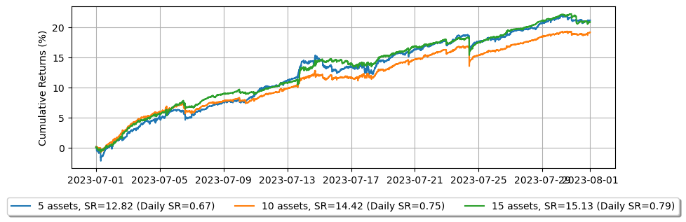
したがって、注文レイテンシを理解することは、より正確なバックテスト結果を達成するために重要です。この理解は、市場メーカーや高頻度トレーダーにとってレイテンシ削減の重要性を強調しています。これが、暗号通貨取引所がメーカーリベートを提供するだけでなく、適格な市場メーカーに低レイテンシのインフラストラクチャを提供する理由です。
よりシンプルなモデル
これまで、\(\xi>0\)の場合のみをカバーしましたが、\(\xi=0\)の場合は、特に暗号通貨では、よりシンプルで実用的です。
Optimal market making の式(4.6)と(4.7)を再確認し、それらが実際のシナリオにどのように適用できるかを探ります。
最適なビッドクォート深度 \(\delta^{b*}_{approx}\) とアスククォート深度 \(\delta^{a*}_{approx}\) は、\(\xi=0\)の場合、公正価格から次のように導出されます:
\begin{align} \delta^{b*}_{approx}(q) = {1 \over k} + {{2q + \Delta} \over 2}\sqrt{{{\gamma \sigma^2 e} \over {2A\Delta k}}} \label{eq4.6}\tag{4.6} \\ \delta^{a*}_{approx}(q) = {1 \over k} - {{2q - \Delta} \over 2}\sqrt{{{\gamma \sigma^2 e} \over {2A\Delta k}}} \label{eq4.7}\tag{4.7} \end{align}
次に、\(c_1\) と \(c_2\) を導入し、平方根からボラティリティ 𝜎 を抽出して定義します:
\begin{align} c_1 = {1 \over k} \\ c_2 = \sqrt{{{\gamma e} \over {2A\Delta k}}} \end{align}
これで、式(4.6)と(4.7)を次のように書き換えることができます:
\begin{align} \delta^{b*}_{approx}(q) = c_1 + {\Delta \over 2} \sigma c_2 + q \sigma c_2 \\ \delta^{a*}_{approx}(q) = c_1 + {\Delta \over 2} \sigma c_2 - q \sigma c_2 \end{align}
これはより簡潔で、\(\gamma\)を調整するだけで済み、その効果はより直接的です。
[13]:
@njit(cache=True)
def compute_coeff_simplified(gamma, delta, A, k):
    inv_k = np.divide(1, k)
    c1 = inv_k
    c2 = np.sqrt(np.divide(gamma * np.exp(1), 2 * A * delta * k))
    return c1, c2

@njit
def gridtrading_glft_mm(hbt, recorder, gamma, order_qty):
    asset_no = 0
    tick_size = hbt.depth(asset_no).tick_size

    arrival_depth = np.full(30_000_000, np.nan, np.float64)
    mid_price_chg = np.full(30_000_000, np.nan, np.float64)

    t = 0
    prev_mid_price_tick = np.nan
    mid_price_tick = np.nan

    tmp = np.zeros(500, np.float64)
    ticks = np.arange(len(tmp)) + 0.5

    A = np.nan
    k = np.nan
    volatility = np.nan
    delta = 1

    grid_num = 20
    max_position = 50 * order_qty

    # Checks every 100 milliseconds.
    while hbt.elapse(100_000_000) == 0:
        #--------------------------------------------------------
        # Records market order's arrival depth from the mid-price.
        if not np.isnan(mid_price_tick):
            depth = -np.inf
            for last_trade in hbt.last_trades(asset_no):
                trade_price_tick = last_trade.px / tick_size

                if last_trade.ev & BUY_EVENT == BUY_EVENT:
                    depth = max(trade_price_tick - mid_price_tick, depth)
                else:
                    depth = max(mid_price_tick - trade_price_tick, depth)
            arrival_depth[t] = depth

        hbt.clear_last_trades(asset_no)
        hbt.clear_inactive_orders(asset_no)

        depth = hbt.depth(asset_no)
        position = hbt.position(asset_no)
        orders = hbt.orders(asset_no)

        best_bid_tick = depth.best_bid_tick
        best_ask_tick = depth.best_ask_tick

        prev_mid_price_tick = mid_price_tick
        mid_price_tick = (best_bid_tick + best_ask_tick) / 2.0

        # Records the mid-price change for volatility calculation.
        mid_price_chg[t] = mid_price_tick - prev_mid_price_tick

        #--------------------------------------------------------
        # Calibrates A, k and calculates the market volatility.

        # Updates A, k, and the volatility every 5-sec.
        if t % 50 == 0:
            # Window size is 10-minute.
            if t >= 6_000 - 1:
                # Calibrates A, k
                tmp[:] = 0
                lambda_ = measure_trading_intensity(arrival_depth[t + 1 - 6_000:t + 1], tmp)
                if len(lambda_) > 2:
                    lambda_ = lambda_[:70] / 600
                    x = ticks[:len(lambda_)]
                    y = np.log(lambda_)
                    k_, logA = linear_regression(x, y)
                    A = np.exp(logA)
                    k = -k_

                # Updates the volatility.
                volatility = np.nanstd(mid_price_chg[t + 1 - 6_000:t + 1]) * np.sqrt(10)

        #--------------------------------------------------------
        # Computes bid price and ask price.

        c1, c2 = compute_coeff_simplified(gamma, delta, A, k)

        half_spread_tick = c1 + delta / 2 * c2 * volatility
        skew = c2 * volatility

        normalized_position = position / order_qty

        reservation_price_tick = mid_price_tick - skew * normalized_position

        bid_price_tick = min(np.round(reservation_price_tick - half_spread_tick), best_bid_tick)
        ask_price_tick = max(np.round(reservation_price_tick + half_spread_tick), best_ask_tick)

        bid_price = bid_price_tick * tick_size
        ask_price = ask_price_tick * tick_size

        grid_interval = max(np.round(half_spread_tick) * tick_size, tick_size)

        bid_price = np.floor(bid_price / grid_interval) * grid_interval
        ask_price = np.ceil(ask_price / grid_interval) * grid_interval

        #--------------------------------------------------------
        # Updates quotes.

        # Creates a new grid for buy orders.
        new_bid_orders = Dict.empty(np.uint64, np.float64)
        if position < max_position and np.isfinite(bid_price):
            for i in range(grid_num):
                bid_price_tick = round(bid_price / tick_size)

                # order price in tick is used as order id.
                new_bid_orders[uint64(bid_price_tick)] = bid_price

                bid_price -= grid_interval

        # Creates a new grid for sell orders.
        new_ask_orders = Dict.empty(np.uint64, np.float64)
        if position > -max_position and np.isfinite(ask_price):
            for i in range(grid_num):
                ask_price_tick = round(ask_price / tick_size)

                # order price in tick is used as order id.
                new_ask_orders[uint64(ask_price_tick)] = ask_price

                ask_price += grid_interval

        order_values = orders.values();
        while order_values.has_next():
            order = order_values.get()
            # Cancels if a working order is not in the new grid.
            if order.cancellable:
                if (
                    (order.side == BUY and order.order_id not in new_bid_orders)
                    or (order.side == SELL and order.order_id not in new_ask_orders)
                ):
                    hbt.cancel(asset_no, order.order_id, False)

        for order_id, order_price in new_bid_orders.items():
            # Posts a new buy order if there is no working order at the price on the new grid.
            if order_id not in orders:
                hbt.submit_buy_order(asset_no, order_id, order_price, order_qty, GTX, LIMIT, False)

        for order_id, order_price in new_ask_orders.items():
            # Posts a new sell order if there is no working order at the price on the new grid.
            if order_id not in orders:
                hbt.submit_sell_order(asset_no, order_id, order_price, order_qty, GTX, LIMIT, False)

        #--------------------------------------------------------
        # Records variables and stats for analysis.

        t += 1

        if t >= len(arrival_depth) or t >= len(mid_price_chg):
            raise Exception

        # Records the current state for stat calculation.
        recorder.record(hbt)
[14]:
def backtest(args):
    asset_name, asset_info = args

    # Obtains the mid-price of the assset to determine the order quantity.
    snapshot = np.load('data/{}_20230630_eod.npz'.format(asset_name))['data']
    best_bid = max(snapshot[snapshot['ev'] & BUY_EVENT == BUY_EVENT]['px'])
    best_ask = min(snapshot[snapshot['ev'] & SELL_EVENT == SELL_EVENT]['px'])
    mid_price = (best_bid + best_ask) / 2.0

    latency_data = np.concatenate(
        [np.load('latency/live_order_latency_{}.npz'.format(date))['data'] for date in range(20230701, 20230732)]
    )

    asset = (
        BacktestAsset()
            .data(['data/{}_{}.npz'.format(asset_name, date) for date in range(20230701, 20230732)])
            .initial_snapshot('data/{}_20230630_eod.npz'.format(asset_name))
            .linear_asset(1.0)
            .intp_order_latency(latency_data)
            .power_prob_queue_model(2.0)
            .no_partial_fill_exchange()
            .trading_value_fee_model(-0.00005, 0.0007)
            .tick_size(asset_info['tick_size'])
            .lot_size(asset_info['lot_size'])
            .roi_lb(0.0)
            .roi_ub(mid_price * 5)
            .last_trades_capacity(10000)
    )

    hbt = ROIVectorMarketDepthBacktest([asset])

    # Sets the order quantity to be equivalent to a notional value of $100.
    order_qty = max(round((100 / mid_price) / asset_info['lot_size']), 1) * asset_info['lot_size']

    recorder = Recorder(1, 30_000_000)

    gamma = 0.00005
    gridtrading_glft_mm(hbt, recorder.recorder, gamma, order_qty)

    hbt.close()

    recorder.to_npz('stats/gridtrading_simple_glft_mm1_{}.npz'.format(asset_name))
[15]:
%%capture
with Pool(16) as p:
    print(p.map(backtest, list(assets.items())))
[16]:
equity_values = {}
for asset_name in assets.keys():
    data = np.load('stats/gridtrading_simple_glft_mm1_{}.npz'.format(asset_name))['0']
    stats = (
        LinearAssetRecord(data)
            .resample('5m')
            .stats()
    )

    equity = stats.entire.with_columns(
        (pl.col('equity_wo_fee') - pl.col('fee')).alias('equity')
    ).select(['timestamp', 'equity'])
    equity_values[asset_name] = equity

fig = plt.figure()
fig.set_size_inches(10, 3)

legend = []
net_equity = None
for i, equity in enumerate(list(equity_values.values())):
    asset_number = i + 1
    if net_equity is None:
        net_equity = equity['equity'].clone()
    else:
        net_equity += equity['equity'].clone()

    if asset_number % 5 == 0:
        # 2_000 is capital for each trading asset.
        net_equity_df = pl.DataFrame({
            'cum_ret': (net_equity / asset_number) / 5_000 * 100,
            'timestamp': equity['timestamp']
        })
        net_equity_rs_df = net_equity_df.group_by_dynamic(
            index_column='timestamp',
            every='1d'
        ).agg([
            pl.col('cum_ret').last()
        ])
        pnl = net_equity_rs_df['cum_ret'].diff()
        sr = pnl.mean() / pnl.std()
        ann_sr = sr * np.sqrt(365)

        plt.plot(net_equity_df['timestamp'], net_equity_df['cum_ret'])
        legend.append('{} assets, SR={:.2f} (Daily SR={:.2f})'.format(asset_number, ann_sr, sr))

plt.legend(
    legend,
    loc='upper center', bbox_to_anchor=(0.5, -0.15),
    fancybox=True, shadow=True, ncol=3
)

plt.grid()
plt.ylabel('Cumulative Returns (%)')
[16]:
Text(0, 0.5, 'Cumulative Returns (%)')
[17]:
def backtest(args):
    asset_name, asset_info = args

    # Obtains the mid-price of the assset to determine the order quantity.
    snapshot = np.load('data/{}_20230630_eod.npz'.format(asset_name))['data']
    best_bid = max(snapshot[snapshot['ev'] & BUY_EVENT == BUY_EVENT]['px'])
    best_ask = min(snapshot[snapshot['ev'] & SELL_EVENT == SELL_EVENT]['px'])
    mid_price = (best_bid + best_ask) / 2.0

    latency_data = np.concatenate(
        [np.load('latency/live_order_latency_{}.npz'.format(date))['data'] for date in range(20230701, 20230732)]
    )

    asset = (
        BacktestAsset()
            .data(['data/{}_{}.npz'.format(asset_name, date) for date in range(20230701, 20230732)])
            .initial_snapshot('data/{}_20230630_eod.npz'.format(asset_name))
            .linear_asset(1.0)
            .intp_order_latency(latency_data)
            .power_prob_queue_model(2.0)
            .no_partial_fill_exchange()
            .trading_value_fee_model(-0.00005, 0.0007)
            .tick_size(asset_info['tick_size'])
            .lot_size(asset_info['lot_size'])
            .roi_lb(0.0)
            .roi_ub(mid_price * 5)
            .last_trades_capacity(10000)
    )

    hbt = ROIVectorMarketDepthBacktest([asset])

    # Sets the order quantity to be equivalent to a notional value of $100.
    order_qty = max(round((100 / mid_price) / asset_info['lot_size']), 1) * asset_info['lot_size']

    recorder = Recorder(1, 30_000_000)

    gamma = 0.001
    gridtrading_glft_mm(hbt, recorder.recorder, gamma, order_qty)

    hbt.close()

    recorder.to_npz('stats/gridtrading_simple_glft_mm2_{}.npz'.format(asset_name))
[18]:
%%capture
with Pool(16) as p:
    print(p.map(backtest, list(assets.items())))
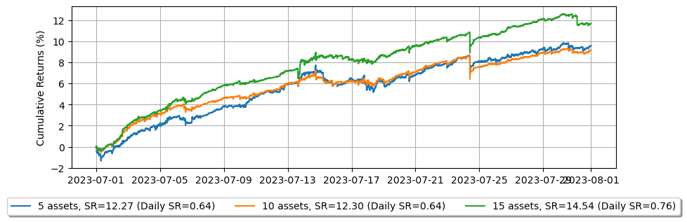
より高い\(\gamma\)では、エクイティカーブにより直線的な線が見られますが、急速に動く市場ではより深刻なドローダウンも経験します。また、スキューが大きいため、ポジションをクローズする傾向が強まり、利益が減少します。
[19]:
equity_values = {}
for asset_name in assets.keys():
    data = np.load('stats/gridtrading_simple_glft_mm2_{}.npz'.format(asset_name))['0']
    stats = (
        LinearAssetRecord(data)
            .resample('5m')
            .stats()
    )

    equity = stats.entire.with_columns(
        (pl.col('equity_wo_fee') - pl.col('fee')).alias('equity')
    ).select(['timestamp', 'equity'])
    equity_values[asset_name] = equity

fig = plt.figure()
fig.set_size_inches(10, 3)

legend = []
net_equity = None
for i, equity in enumerate(list(equity_values.values())):
    asset_number = i + 1
    if net_equity is None:
        net_equity = equity['equity'].clone()
    else:
        net_equity += equity['equity'].clone()

    if asset_number % 5 == 0:
        # 2_000 is capital for each trading asset.
        net_equity_df = pl.DataFrame({
            'cum_ret': (net_equity / asset_number) / 5_000 * 100,
            'timestamp': equity['timestamp']
        })
        net_equity_rs_df = net_equity_df.group_by_dynamic(
            index_column='timestamp',
            every='1d'
        ).agg([
            pl.col('cum_ret').last()
        ])
        pnl = net_equity_rs_df['cum_ret'].diff()
        sr = pnl.mean() / pnl.std()
        ann_sr = sr * np.sqrt(365)

        plt.plot(net_equity_df['timestamp'], net_equity_df['cum_ret'])
        legend.append('{} assets, SR={:.2f} (Daily SR={:.2f})'.format(asset_number, ann_sr, sr))

plt.legend(
    legend,
    loc='upper center', bbox_to_anchor=(0.5, -0.15),
    fancybox=True, shadow=True, ncol=3
)

plt.grid()
plt.ylabel('Cumulative Returns (%)')
[19]:
Text(0, 0.5, 'Cumulative Returns (%)')
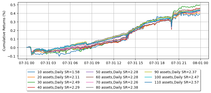
より多くの資産のケース
市場を作る資産が多いほど、リスク調整後のリターンが向上します。この効果は劇的に明らかになります。
[20]:
def backtest(args):
    asset_name, asset_info = args

    # Obtains the mid-price of the assset to determine the order quantity.
    snapshot = np.load('data/{}_20230730_eod.npz'.format(asset_name))['data']
    best_bid = max(snapshot[snapshot['ev'] & BUY_EVENT == BUY_EVENT]['px'])
    best_ask = min(snapshot[snapshot['ev'] & SELL_EVENT == SELL_EVENT]['px'])
    mid_price = (best_bid + best_ask) / 2.0

    latency_data = np.concatenate(
        [np.load('latency/live_order_latency_{}.npz'.format(date))['data'] for date in range(20230731, 20230732)]
    )

    asset = (
        BacktestAsset()
            .data(['data/{}_{}.npz'.format(asset_name, date) for date in range(20230731, 20230732)])
            .initial_snapshot('data/{}_20230730_eod.npz'.format(asset_name))
            .linear_asset(1.0)
            .intp_order_latency(latency_data)
            .power_prob_queue_model(2.0)
            .no_partial_fill_exchange()
            .trading_value_fee_model(-0.00005, 0.0007)
            .tick_size(asset_info['tick_size'])
            .lot_size(asset_info['lot_size'])
            .roi_lb(0.0)
            .roi_ub(mid_price * 5)
            .last_trades_capacity(10000)
    )

    hbt = ROIVectorMarketDepthBacktest([asset])

    # Sets the order quantity to be equivalent to a notional value of $100.
    order_qty = max(round((100 / mid_price) / asset_info['lot_size']), 1) * asset_info['lot_size']

    recorder = Recorder(1, 30_000_000)

    gamma = 0.00005
    gridtrading_glft_mm(hbt, recorder.recorder, gamma, order_qty)

    hbt.close()

    recorder.to_npz('stats/gridtrading_simple_glft_mm3_{}.npz'.format(asset_name))
[21]:
%%capture
with open('assets2.json', 'r') as f:
    assets = json.load(f)

with Pool(16) as p:
    print(p.map(backtest, list(assets.items())))
[22]:
equity_values = {}
sr_values = {}

np.seterr(divide='ignore', invalid='ignore')

for asset_name in assets.keys():
    data = np.load('stats/gridtrading_simple_glft_mm3_{}.npz'.format(asset_name))['0']
    stats = (
        LinearAssetRecord(data)
            .resample('5m')
            .stats()
    )

    equity = stats.entire.with_columns(
        (pl.col('equity_wo_fee') - pl.col('fee')).alias('equity')
    ).select(['timestamp', 'equity'])

    pnl = equity['equity'].diff()
    sr = np.divide(pnl.mean(), pnl.std())

    equity_values[asset_name] = equity
    sr_values[asset_name] = sr

sr_m = np.nanmean(list(sr_values.values()))
sr_s = np.nanstd(list(sr_values.values()))

fig = plt.figure()
fig.set_size_inches(10, 3)

legend = []
asset_number = 0
net_equity = None
for i, (equity, sr) in enumerate(zip(equity_values.values(), sr_values.values())):
    # There are some assets that aren't working within this scheme.
    # This might be because the order arrivals don't follow a Poisson distribution that this model assumes.
    # As a result, it filters out assets whose SR falls outside -0.5 sigma.
    if (sr - sr_m) / sr_s > -0.5:
        asset_number += 1
        if net_equity is None:
            net_equity = equity.clone()
        else:
            net_equity = net_equity.select(
                'timestamp',
                (pl.col('equity') + equity['equity']).alias('equity')
            )

        if asset_number % 10 == 0:
            # 5_000 is capital for each trading asset.
            net_equity_ = net_equity['equity'] / asset_number / 5_000
            pnl = net_equity_.diff()
            # Since the P&L is resampled at a 5-minute interval
            sr = pnl.mean() / pnl.std() * np.sqrt(24 * 60 / 5)
            legend.append('{} assets,Daily SR={:.2f}'.format(asset_number, sr))
            plt.plot(net_equity['timestamp'], net_equity_ * 100)

plt.legend(
    legend,
    loc='upper center', bbox_to_anchor=(0.5, -0.15),
    fancybox=True, shadow=True, ncol=3
)

plt.grid()
plt.ylabel('Cumulative Returns (%)')
[22]:
Text(0, 0.5, 'Cumulative Returns (%)')