Guéant–Lehalle–Fernandez-Tapia マーケットメークとグリッドトレード
概要
グリッドトレーディングはシンプルで理解しやすく、高頻度環境で優れています。しかし、高頻度取引の複雑さを考えると、理想的なスプレッド、注文間隔、スキューを最適化することは困難です。さらに、これらの値は市場の状況に応じて変動するため、固定された設定は最適ではありません。
グリッドトレーディングの適応性を向上させるための1つの解決策は、よく開発されたマーケットメイキングモデルと組み合わせることです。これがどのように実現できるかを見てみましょう。
Guéant–Lehalle–Fernandez-Tapia マーケットメイキングモデル
このモデルは、よく知られたアベラネダ・ストイコビッチモデルの進化形であり、終端時間Tの漸近的な挙動の閉形式近似を提供します。簡単に言えば、このモデルは終端時間を指定しないため、典型的な株式、スポット資産、または暗号通貨の永久契約に適しています。このモデルを使用することで、市場の状況に応じてハーフスプレッドとスキューが正確に調整されることが期待されます。
この分析では、Optimal market making の式(4.6)と(4.7)に焦点を当て、それらが実際のシナリオにどのように適用できるかを探ります。
最適なビッドクォート深度 \(\delta^{b*}_{approx}\) とアスククォート深度 \(\delta^{a*}_{approx}\) は、公正価格から次のように導出されます:
\begin{align} \delta^{b*}_{approx}(q) = {1 \over {\xi \Delta}}log(1 + {\xi \Delta \over k}) + {{2q + \Delta} \over 2}\sqrt{{{\gamma \sigma^2} \over {2A\Delta k}}(1 + {\xi \Delta \over k})^{{k \over {\xi \Delta}} + 1}} \label{eq4.6}\tag{4.6} \\ \delta^{a*}_{approx}(q) = {1 \over {\xi \Delta}}log(1 + {\xi \Delta \over k}) - {{2q - \Delta} \over 2}\sqrt{{{\gamma \sigma^2} \over {2A\Delta k}}(1 + {\xi \Delta \over k})^{{k \over {\xi \Delta}} + 1}} \label{eq4.7}\tag{4.7} \end{align}
次に、\(c_1\) と \(c_2\) を導入し、平方根からボラティリティ 𝜎 を抽出して定義します:
\begin{align} c_1 = {1 \over {\xi \Delta}}log(1 + {\xi \Delta \over k}) \\ c_2 = \sqrt{{\gamma \over {2A\Delta k}}(1 + {\xi \Delta \over k})^{{k \over {\xi \Delta}} + 1}} \end{align}
これで、式(4.6)と(4.7)を次のように書き換えることができます:
\begin{align} \delta^{b*}_{approx}(q) = c_1 + {\Delta \over 2} \sigma c_2 + q \sigma c_2 \\ \delta^{a*}_{approx}(q) = c_1 + {\Delta \over 2} \sigma c_2 - q \sigma c_2 \end{align}
ご覧のとおり、これはハーフスプレッドとスキューで構成されています。\(q\) はマーケットメイカーの在庫(ポジション)を表します。
\begin{align} \text{half spread} = C_1 + {\Delta \over 2} \sigma C_2 \\ \text{skew} = \sigma C_2 \\ \delta^{b*}_{approx}(q) = \text{half spread} + \text{skew} \times q \\ \delta^{a*}_{approx}(q) = \text{half spread} - \text{skew} \times q \end{align}
したがって、
\begin{align} \text{bid price} = \text{fair price} - (\text{half spread} + \text{skew} \times q) \\ \text{ask price} = \text{fair price} + (\text{half spread} - \text{skew} \times q) \end{align}
取引強度の計算
最適なクォートを決定するためには、\(c_1\) と \(c_2\) を計算する必要があります。そのためには、取引強度の \(A\) と \(k\) をキャリブレーションし、市場のボラティリティ \(\sigma\) を計算する必要があります。
取引強度は次のように定義されます:
これらの値を市場データを使用してキャリブレーションします。詳細はこの記事をご覧ください。そのためには、市場注文の到着を記録する必要があります。
私たちのマーケットメイカーは100msごとに反応し、この間隔で注文を投稿またはキャンセルします。したがって、クォートの取引強度も同じタイムステップで測定されます。理想的には、注文のキュー位置も考慮する必要がありますが、この分析では問題を単純化するために注文キュー位置は考慮しません。
[ ]:
import numpy as np
from numba import njit

from hftbacktest import BUY_EVENT


@njit
def measure_trading_intensity_and_volatility(hbt):
    tick_size = hbt.depth(0).tick_size
    arrival_depth = np.full(10_000_000, np.nan, np.float64)
    mid_price_chg = np.full(10_000_000, np.nan, np.float64)

    t = 0
    prev_mid_price_tick = np.nan
    mid_price_tick = np.nan

    # Checks every 100 milliseconds.
    while hbt.elapse(100_000_000) == 0:
        # --------------------------------------------------------
        # Records market order's arrival depth from the mid-price.
        if not np.isnan(mid_price_tick):
            depth = -np.inf
            for last_trade in hbt.last_trades(0):
                trade_price_tick = last_trade.px / tick_size

                if last_trade.ev & BUY_EVENT == BUY_EVENT:
                    depth = np.nanmax([trade_price_tick - mid_price_tick, depth])
                else:
                    depth = np.nanmax([mid_price_tick - trade_price_tick, depth])
            arrival_depth[t] = depth

        hbt.clear_last_trades(0)

        depth = hbt.depth(0)

        best_bid_tick = depth.best_bid_tick
        best_ask_tick = depth.best_ask_tick

        prev_mid_price_tick = mid_price_tick
        mid_price_tick = (best_bid_tick + best_ask_tick) / 2.0

        # Records the mid-price change for volatility calculation.
        mid_price_chg[t] = mid_price_tick - prev_mid_price_tick

        t += 1
        if t >= len(arrival_depth) or t >= len(mid_price_chg):
            raise Exception
    return arrival_depth[:t], mid_price_chg[:t]
取引強度を測定する際に注文のキュー位置を考慮しないため、クォートをクロスする市場取引のみが実行されたと見なされます。
[ ]:
@njit
def measure_trading_intensity(order_arrival_depth, out):
    max_tick = 0
    for depth in order_arrival_depth:
        if not np.isfinite(depth):
            continue

        # Sets the tick index to 0 for the nearest possible best price
        # as the order arrival depth in ticks is measured from the mid-price
        tick = round(depth / 0.5) - 1

        # In a fast-moving market, buy trades can occur below the mid-price (and vice versa for sell trades)
        # since the mid-price is measured in a previous time-step;
        # however, to simplify the problem, we will exclude those cases.
        if tick < 0 or tick >= len(out):
            continue

        # All of our possible quotes within the order arrival depth,
        # excluding those at the same price, are considered executed.
        out[:tick] += 1

        max_tick = max(max_tick, tick)
    return out[:max_tick]
HftBacktestを実行して市場を再生し、注文到着深度と価格変動を記録します。
[ ]:
from hftbacktest import BacktestAsset, ROIVectorMarketDepthBacktest

asset = (
    BacktestAsset()
    .data(["data/ethusdt_20221003.npz"])
    .initial_snapshot("data/ethusdt_20221002_eod.npz")
    .linear_asset(1.0)
    .intp_order_latency(["latency/feed_latency_20221003.npz"])
    .power_prob_queue_model(2.0)
    .no_partial_fill_exchange()
    .trading_value_fee_model(-0.00005, 0.0007)
    .tick_size(0.01)
    .lot_size(0.001)
    .roi_lb(0.0)
    .roi_ub(3000.0)
    .last_trades_capacity(10000)
)

hbt = ROIVectorMarketDepthBacktest([asset])

arrival_depth, mid_price_chg = measure_trading_intensity_and_volatility(hbt)

_ = hbt.close()
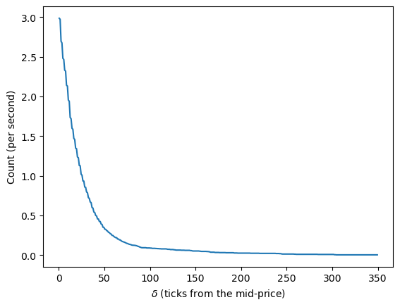
記録された注文到着深度から取引強度を測定し、プロットします。
[ ]:
tmp = np.zeros(500, np.float64)

# Measures trading intensity (lambda) for the first 10-minute window.
lambda_ = measure_trading_intensity(arrival_depth[:6_000], tmp)

# Since it is measured for a 10-minute window, divide by 600 to convert it to per second.
lambda_ /= 600

# Creates ticks from the mid-price.
ticks = np.arange(len(lambda_)) + 0.5
[ ]:
from matplotlib import pyplot as plt

plt.plot(ticks, lambda_)
plt.xlabel("$ \delta $ (ticks from the mid-price)")
plt.ylabel("Count (per second)")
Text(0, 0.5, 'Count (per second)')
線形回帰を使用して \(A\) と \(k\) をキャリブレーションします。両辺の対数を取ると、\(log \lambda = -k \delta + logA\) となります。
[ ]:
@njit
def linear_regression(x, y):
    sx = np.sum(x)
    sy = np.sum(y)
    sx2 = np.sum(x**2)
    sxy = np.sum(x * y)
    w = len(x)
    slope = (w * sxy - sx * sy) / (w * sx2 - sx**2)
    intercept = (sy - slope * sx) / w
    return slope, intercept
[ ]:
y = np.log(lambda_)
k_, logA = linear_regression(ticks, y)
A = np.exp(logA)
k = -k_

print("A={}, k={}".format(A, k))
A=0.8426573649994981, k=0.016958811558646644
[ ]:
plt.plot(lambda_)
plt.plot(A * np.exp(-k * ticks))
plt.xlabel("$ \delta $ (ticks from the mid-price)")
plt.ylabel("Count (per second)")
plt.legend(["Actual", "Fitted curve"])
<matplotlib.legend.Legend at 0x7fac86b74760>
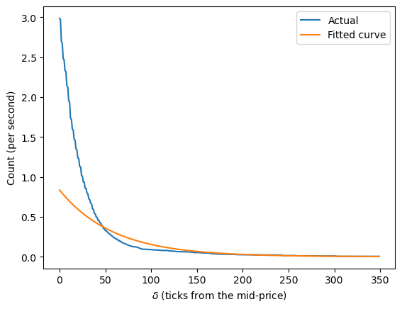
ご覧のとおり、フィットされたラムダ関数は全範囲で正確ではありません。特に、ミッドプライスに近い浅い範囲では取引強度を過大評価し、ミッドプライスから離れた深い範囲では過小評価します。
私たちのクォートは、少なくとも典型的な市場条件下(高ボラティリティ条件を除く)では、ミッドプライスに近い範囲に配置される可能性が高いため、特に最も近い範囲に対して関数を再フィットします。
[ ]:
# Refits for the range un to 70 ticks.
x_shallow = ticks[:70]
lambda_shallow = lambda_[:70]

y = np.log(lambda_shallow)
k_, logA = linear_regression(x_shallow, y)
A = np.exp(logA)
k = -k_

print("A={}, k={}".format(A, k))
A=2.986162360812285, k=0.04235741115084049
[ ]:
plt.plot(lambda_shallow)
plt.plot(A * np.exp(-k * x_shallow))
plt.xlabel("$ \delta $ (ticks from the mid-price)")
plt.ylabel("Count (per second)")
plt.legend(["Actual", "Fitted curve"])
<matplotlib.legend.Legend at 0x7fac86b77070>
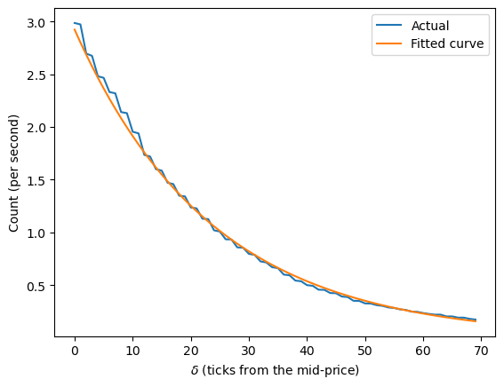
これで、より正確な取引強度関数が得られました。次に、クォートがどこに配置されるかを見てみましょう。
その前に、まずボラティリティを計算しましょう。
[ ]:
# Since we need volatility in ticks per square root of a second and our measurement is every 100ms,
# multiply by the square root of 10.
volatility = np.nanstd(mid_price_chg) * np.sqrt(10)
print(volatility)
10.725509539115974
式に従って \(c_1\) と \(c_2\) を計算します。
[ ]:
@njit
def compute_coeff(xi, gamma, delta, A, k):
    inv_k = np.divide(1, k)
    c1 = 1 / (xi * delta) * np.log(1 + xi * delta * inv_k)
    c2 = np.sqrt(
        np.divide(gamma, 2 * A * delta * k)
        * ((1 + xi * delta * inv_k) ** (k / (xi * delta) + 1))
    )
    return c1, c2
Guéant–Lehalle–Fernandez-Tapia の式では、\(\Delta = 1\) および \(\xi = \gamma\) です。\(\gamma\) の値は任意に選択されます。
[ ]:
gamma = 0.05
delta = 1
volatility = 10.69

c1, c2 = compute_coeff(gamma, gamma, delta, A, k)

half_spread_tick = 1 * c1 + 1 / 2 * c2 * volatility
skew = c2 * volatility
print("half_spread_tick={}, skew={}".format(half_spread_tick, skew))
half_spread_tick=20.47208533844371, skew=9.76326865029227
クォートがミッドプライスから20ティック離れている場合、それは何を意味しますか?記録された注文到着深度を分析することで、マーケットメイカーとして参加する市場取引の数を特定できます。これは数量ではなくカウントで測定されます。また、スキューが非常に強いことがわかります。2つのポジションを積み上げるだけで、全体のハーフスプレッドがオフセットされます。
[ ]:
from scipy import stats

# inverse of percentile
pct = stats.percentileofscore(
    arrival_depth[np.isfinite(arrival_depth)], half_spread_tick
)
your_pct = 100 - pct
print("{:.2f}%".format(your_pct))
1.86%
特定のタイムステップごとに市場取引の約1.86%がクォートを実行する可能性があります。これは取引数量の割合ではないことに注意してください。
モデルを使用したマーケットメイカーの実装
注: この例は教育目的のみであり、高頻度マーケットメイキングスキームの効果的な戦略を示しています。すべてのバックテストは、Binance Futuresで利用可能な最高のマーケットメイカーリベートである0.005%のリベートに基づいています。詳細については、Binance Upgrades USDⓢ-Margined Futures Liquidity Provider Program を参照してください。
この例では、予測項を無視し、公正価格がミッドプライスと等しいと仮定します。短期的には内在価値が安定していると予想されるためです。
[ ]:
from numba.typed import Dict

from hftbacktest import BUY, GTX, LIMIT, SELL
from hftbacktest import BUY, GTX, LIMIT, SELL
from hftbacktest import BUY, GTX, LIMIT, SELL
from hftbacktest import BUY, GTX, LIMIT, SELL
from hftbacktest import BUY, GTX, LIMIT, SELL
from hftbacktest import BUY, GTX, LIMIT, SELL
from hftbacktest import BUY, GTX, LIMIT, SELL
from hftbacktest import BUY, GTX, LIMIT, SELL
from hftbacktest import BUY, GTX, LIMIT, SELL
from hftbacktest import BUY, GTX, LIMIT, SELL
from hftbacktest import BUY, GTX, LIMIT, SELL
from hftbacktest import BUY, GTX, LIMIT, SELL
from hftbacktest import BUY, GTX, LIMIT, SELL
from hftbacktest import BUY, GTX, LIMIT, SELL
from hftbacktest import BUY, GTX, LIMIT, SELL
from hftbacktest import BUY, GTX, LIMIT, SELL
from hftbacktest import BUY, GTX, LIMIT, SELL
from hftbacktest import BUY, GTX, LIMIT, SELL
from hftbacktest import BUY, GTX, LIMIT, SELL
from hftbacktest import BUY, GTX, LIMIT, SELL
from hftbacktest import BUY, GTX, LIMIT, SELL
from hftbacktest import BUY, GTX, LIMIT, SELL
from hftbacktest import BUY, GTX, LIMIT, SELL
from hftbacktest import BUY, GTX, LIMIT, SELL
from hftbacktest import BUY, GTX, LIMIT, SELL
from hftbacktest import BUY, GTX, LIMIT, SELL
from hftbacktest import BUY, GTX, LIMIT, SELL
from hftbacktest import BUY, GTX, LIMIT, SELL
from hftbacktest import BUY, GTX, LIMIT, SELL
from hftbacktest import BUY, GTX, LIMIT, SELL

out_dtype = np.dtype(
    [
        ("half_spread_tick", "f8"),
        ("skew", "f8"),
        ("volatility", "f8"),
        ("A", "f8"),
        ("k", "f8"),
    ]
)


@njit
def glft_market_maker(hbt, recorder):
    tick_size = hbt.depth(0).tick_size
    arrival_depth = np.full(10_000_000, np.nan, np.float64)
    mid_price_chg = np.full(10_000_000, np.nan, np.float64)
    out = np.zeros(10_000_000, out_dtype)

    t = 0
    prev_mid_price_tick = np.nan
    mid_price_tick = np.nan

    tmp = np.zeros(500, np.float64)
    ticks = np.arange(len(tmp)) + 0.5

    A = np.nan
    k = np.nan
    volatility = np.nan
    gamma = 0.05
    delta = 1

    order_qty = 1
    max_position = 20

    # Checks every 100 milliseconds.
    while hbt.elapse(100_000_000) == 0:
        # --------------------------------------------------------
        # Records market order's arrival depth from the mid-price.
        if not np.isnan(mid_price_tick):
            depth = -np.inf
            for last_trade in hbt.last_trades(0):
                trade_price_tick = last_trade.px / tick_size

                if last_trade.ev & BUY_EVENT == BUY_EVENT:
                    depth = np.nanmax([trade_price_tick - mid_price_tick, depth])
                else:
                    depth = np.nanmax([mid_price_tick - trade_price_tick, depth])
            arrival_depth[t] = depth

        hbt.clear_last_trades(0)
        hbt.clear_inactive_orders(0)

        depth = hbt.depth(0)
        position = hbt.position(0)
        orders = hbt.orders(0)

        best_bid_tick = depth.best_bid_tick
        best_ask_tick = depth.best_ask_tick

        prev_mid_price_tick = mid_price_tick
        mid_price_tick = (best_bid_tick + best_ask_tick) / 2.0

        # Records the mid-price change for volatility calculation.
        mid_price_chg[t] = mid_price_tick - prev_mid_price_tick

        # --------------------------------------------------------
        # Calibrates A, k and calculates the market volatility.

        # Updates A, k, and the volatility every 5-sec.
        if t % 50 == 0:
            # Window size is 10-minute.
            if t >= 6_000 - 1:
                # Calibrates A, k
                tmp[:] = 0
                lambda_ = measure_trading_intensity(
                    arrival_depth[t + 1 - 6_000 : t + 1], tmp
                )
                if len(lambda_) > 2:
                    lambda_ = lambda_[:70] / 600
                    x = ticks[: len(lambda_)]
                    y = np.log(lambda_)
                    k_, logA = linear_regression(x, y)
                    A = np.exp(logA)
                    k = -k_

                # Updates the volatility.
                volatility = np.nanstd(mid_price_chg[t + 1 - 6_000 : t + 1]) * np.sqrt(
                    10
                )

        # --------------------------------------------------------
        # Computes bid price and ask price.

        c1, c2 = compute_coeff(gamma, gamma, delta, A, k)

        half_spread_tick = c1 + delta / 2 * c2 * volatility
        skew = c2 * volatility

        reservation_price_tick = mid_price_tick - skew * position

        bid_price_tick = np.minimum(
            np.round(reservation_price_tick - half_spread_tick), best_bid_tick
        )
        ask_price_tick = np.maximum(
            np.round(reservation_price_tick + half_spread_tick), best_ask_tick
        )

        bid_price = bid_price_tick * tick_size
        ask_price = ask_price_tick * tick_size

        # --------------------------------------------------------
        # Updates quotes.

        # Cancel orders if they differ from the updated bid and ask prices.
        order_values = orders.values()
        while order_values.has_next():
            order = order_values.get()
            # Cancels if a working order is not in the new grid.
            if order.cancellable:
                if (order.side == BUY and order.price != bid_price) or (
                    order.side == SELL and order.price != ask_price
                ):
                    hbt.cancel(0, order.order_id, False)

        # If the current position is within the maximum position,
        # submit the new order only if no order exists at the same price.
        if position < max_position and np.isfinite(bid_price):
            bid_price_as_order_id = round(bid_price / tick_size)
            if bid_price_as_order_id not in orders:
                hbt.submit_buy_order(
                    0, bid_price_as_order_id, bid_price, order_qty, GTX, LIMIT, False
                )
        if position > -max_position and np.isfinite(ask_price):
            ask_price_as_order_id = round(ask_price / tick_size)
            if ask_price_as_order_id not in orders:
                hbt.submit_sell_order(
                    0, ask_price_as_order_id, ask_price, order_qty, GTX, LIMIT, False
                )

        # --------------------------------------------------------
        # Records variables and stats for analysis.

        out[t].half_spread_tick = half_spread_tick
        out[t].skew = skew
        out[t].volatility = volatility
        out[t].A = A
        out[t].k = k

        t += 1

        if t >= len(arrival_depth) or t >= len(mid_price_chg) or t >= len(out):
            raise Exception

        # Records the current state for stat calculation.
        recorder.record(hbt)
    return out[:t]
[ ]:
from hftbacktest import Recorder
from hftbacktest.stats import LinearAssetRecord

asset = (
    BacktestAsset()
    .data(["data/ethusdt_20221003.npz"])
    .initial_snapshot("data/ethusdt_20221002_eod.npz")
    .linear_asset(1.0)
    .intp_order_latency(["latency/feed_latency_20221003.npz"])
    .power_prob_queue_model(2.0)
    .no_partial_fill_exchange()
    .trading_value_fee_model(-0.00005, 0.0007)
    .tick_size(0.01)
    .lot_size(0.001)
    .roi_lb(0.0)
    .roi_ub(3000.0)
    .last_trades_capacity(10000)
)

hbt = ROIVectorMarketDepthBacktest([asset])

recorder = Recorder(1, 5_000_000)

out = glft_market_maker(hbt, recorder.recorder)

hbt.close()

stats = LinearAssetRecord(recorder.get(0)).stats(book_size=30_000)
stats.summary()
| start | end | SR | Sortino | Return | MaxDrawdown | DailyNumberOfTrades | DailyTurnover | ReturnOverMDD | ReturnOverTrade | MaxPositionValue |
|---|---|---|---|---|---|---|---|---|---|---|
| datetime[μs] | datetime[μs] | f64 | f64 | f64 | f64 | f64 | f64 | f64 | f64 | f64 |
| 2022-10-03 00:00:00 | 2022-10-03 23:59:50 | -246.379582 | -264.130529 | -0.020574 | 0.020601 | 13579.57171 | 590.242857 | -0.998715 | -0.000035 | 19790.625 |
[17]:
stats.plot()

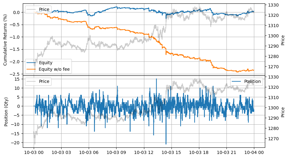
[18]:
stats.plot()
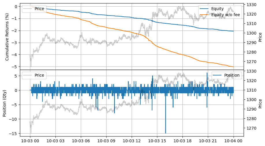
調整係数
スキューが強すぎるように見えるため、マーケットメイカーはポジションを取ることに消極的です。スキューを緩和するために、計算されたハーフスプレッドとスキューに調整係数 \(adj_1\) と \(adj_2\) を導入します。
[ ]:
from numba.typed import Dict


@njit
def glft_market_maker(hbt, recorder):
    tick_size = hbt.depth(0).tick_size
    arrival_depth = np.full(10_000_000, np.nan, np.float64)
    mid_price_chg = np.full(10_000_000, np.nan, np.float64)
    out = np.zeros(10_000_000, out_dtype)

    t = 0
    prev_mid_price_tick = np.nan
    mid_price_tick = np.nan

    tmp = np.zeros(500, np.float64)
    ticks = np.arange(len(tmp)) + 0.5

    A = np.nan
    k = np.nan
    volatility = np.nan
    gamma = 0.05
    delta = 1
    adj1 = 1
    adj2 = 0.05  # Uses the same value as gamma.

    order_qty = 1
    max_position = 20

    # Checks every 100 milliseconds.
    while hbt.elapse(100_000_000) == 0:
        # --------------------------------------------------------
        # Records market order's arrival depth from the mid-price.
        if not np.isnan(mid_price_tick):
            depth = -np.inf
            for last_trade in hbt.last_trades(0):
                trade_price_tick = last_trade.px / tick_size

                if last_trade.ev & BUY_EVENT == BUY_EVENT:
                    depth = np.nanmax([trade_price_tick - mid_price_tick, depth])
                else:
                    depth = np.nanmax([mid_price_tick - trade_price_tick, depth])
            arrival_depth[t] = depth

        hbt.clear_last_trades(0)
        hbt.clear_inactive_orders(0)

        depth = hbt.depth(0)
        position = hbt.position(0)
        orders = hbt.orders(0)

        best_bid_tick = depth.best_bid_tick
        best_ask_tick = depth.best_ask_tick

        prev_mid_price_tick = mid_price_tick
        mid_price_tick = (best_bid_tick + best_ask_tick) / 2.0

        # Records the mid-price change for volatility calculation.
        mid_price_chg[t] = mid_price_tick - prev_mid_price_tick

        # --------------------------------------------------------
        # Calibrates A, k and calculates the market volatility.

        # Updates A, k, and the volatility every 5-sec.
        if t % 50 == 0:
            # Window size is 10-minute.
            if t >= 6_000 - 1:
                # Calibrates A, k
                tmp[:] = 0
                lambda_ = measure_trading_intensity(
                    arrival_depth[t + 1 - 6_000 : t + 1], tmp
                )
                if len(lambda_) > 2:
                    lambda_ = lambda_[:70] / 600
                    x = ticks[: len(lambda_)]
                    y = np.log(lambda_)
                    k_, logA = linear_regression(x, y)
                    A = np.exp(logA)
                    k = -k_

                # Updates the volatility.
                volatility = np.nanstd(mid_price_chg[t + 1 - 6_000 : t + 1]) * np.sqrt(
                    10
                )

        # --------------------------------------------------------
        # Computes bid price and ask price.

        c1, c2 = compute_coeff(gamma, gamma, delta, A, k)

        half_spread_tick = (c1 + delta / 2 * c2 * volatility) * adj1
        skew = c2 * volatility * adj2

        reservation_price_tick = mid_price_tick - skew * position

        bid_price_tick = np.minimum(
            np.round(reservation_price_tick - half_spread_tick), best_bid_tick
        )
        ask_price_tick = np.maximum(
            np.round(reservation_price_tick + half_spread_tick), best_ask_tick
        )

        bid_price = bid_price_tick * tick_size
        ask_price = ask_price_tick * tick_size

        # --------------------------------------------------------
        # Updates quotes.

        # Cancel orders if they differ from the updated bid and ask prices.
        order_values = orders.values()
        while order_values.has_next():
            order = order_values.get()
            # Cancels if a working order is not in the new grid.
            if order.cancellable:
                if (order.side == BUY and order.price_tick != bid_price_tick) or (
                    order.side == SELL and order.price_tick != ask_price_tick
                ):
                    hbt.cancel(0, order.order_id, False)

        # If the current position is within the maximum position,
        # submit the new order only if no order exists at the same price.
        if position < max_position and np.isfinite(bid_price):
            bid_price_as_order_id = round(bid_price / tick_size)
            if bid_price_as_order_id not in orders:
                hbt.submit_buy_order(
                    0, bid_price_as_order_id, bid_price, order_qty, GTX, LIMIT, False
                )
        if position > -max_position and np.isfinite(ask_price):
            ask_price_as_order_id = round(ask_price / tick_size)
            if ask_price_as_order_id not in orders:
                hbt.submit_sell_order(
                    0, ask_price_as_order_id, ask_price, order_qty, GTX, LIMIT, False
                )

        # --------------------------------------------------------
        # Records variables and stats for analysis.

        out[t].half_spread_tick = half_spread_tick
        out[t].skew = skew
        out[t].volatility = volatility
        out[t].A = A
        out[t].k = k

        t += 1

        if t >= len(arrival_depth) or t >= len(mid_price_chg) or t >= len(out):
            raise Exception

        # Records the current state for stat calculation.
        recorder.record(hbt)
    return out[:t]
[ ]:
asset = (
    BacktestAsset()
    .data(["data/ethusdt_20221003.npz"])
    .initial_snapshot("data/ethusdt_20221002_eod.npz")
    .linear_asset(1.0)
    .intp_order_latency(["latency/feed_latency_20221003.npz"])
    .power_prob_queue_model(2.0)
    .no_partial_fill_exchange()
    .trading_value_fee_model(-0.00005, 0.0007)
    .tick_size(0.01)
    .lot_size(0.001)
    .roi_lb(0.0)
    .roi_ub(3000.0)
    .last_trades_capacity(10000)
)

hbt = ROIVectorMarketDepthBacktest([asset])

recorder = Recorder(1, 5_000_000)

out = glft_market_maker(hbt, recorder.recorder)

hbt.close()

stats = LinearAssetRecord(recorder.get(0)).stats(book_size=30_000)
stats.summary()
| start | end | SR | Sortino | Return | MaxDrawdown | DailyNumberOfTrades | DailyTurnover | ReturnOverMDD | ReturnOverTrade | MaxPositionValue |
|---|---|---|---|---|---|---|---|---|---|---|
| datetime[μs] | datetime[μs] | f64 | f64 | f64 | f64 | f64 | f64 | f64 | f64 | f64 |
| 2022-10-03 00:00:00 | 2022-10-03 23:59:50 | 1.202048 | 1.471295 | 0.000359 | 0.004763 | 10987.271675 | 477.498424 | 0.075478 | 7.5295e-7 | 27563.655 |
[21]:
stats.plot()
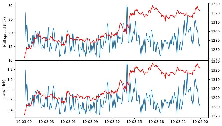
改善されましたが、リベートを考慮しても、せいぜい損益分岐点に達するだけです。以下に示すように、ハーフスプレッドとスキューは主に \(c_2\) と市場のボラティリティに影響されて一緒に動きます。
[ ]:
import polars as pl

records = recorder.get(0)
df = (
    pl.DataFrame(out)
    .with_columns(
        pl.Series("timestamp", records["timestamp"]),
        pl.Series("price", records["price"]),
    )
    .with_columns(pl.from_epoch("timestamp", time_unit="ns"))
)

df = df.group_by_dynamic("timestamp", every="5m").agg(
    pl.col("price").last(),
    pl.col("half_spread_tick").last(),
    pl.col("skew").last(),
    pl.col("volatility").last(),
    pl.col("A").last(),
    pl.col("k").last(),
)

fig, (ax1, ax2) = plt.subplots(2, 1, sharex=True)
fig.subplots_adjust(hspace=0)
fig.set_size_inches(10, 6)

ax1.plot(df["timestamp"], df["half_spread_tick"])
ax1.twinx().plot(df["timestamp"], df["price"], "r")
ax1.set_ylabel("Half spread (tick)")

ax2.plot(df["timestamp"], df["skew"])
ax2.twinx().plot(df["timestamp"], df["price"], "r")
ax2.set_ylabel("Skew (tick)")
Text(0, 0.5, 'Skew (tick)')
[ ]:
fig, (ax1, ax2, ax3) = plt.subplots(3, 1, sharex=True)
fig.subplots_adjust(hspace=0)
fig.set_size_inches(10, 9)
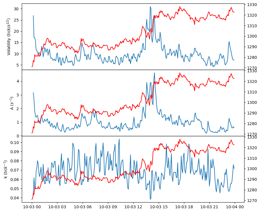
ax1.plot(df["timestamp"], df["volatility"])
ax1.twinx().plot(df["timestamp"], df["price"], "r")
ax1.set_ylabel("Volatility ($ tick/s^{1/2} $)")
ax2.plot(df["timestamp"], df["A"])
ax2.twinx().plot(df["timestamp"], df["price"], "r")
ax2.set_ylabel("A ($ s^{-1} $)")
ax3.plot(df["timestamp"], df["k"])
ax3.twinx().plot(df["timestamp"], df["price"], "r")
ax3.set_ylabel("k ($ tick^{-1} $)")
Text(0, 0.5, 'k ($ tick^{-1} $)')
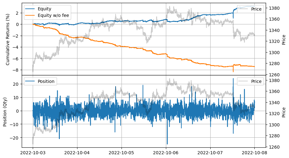
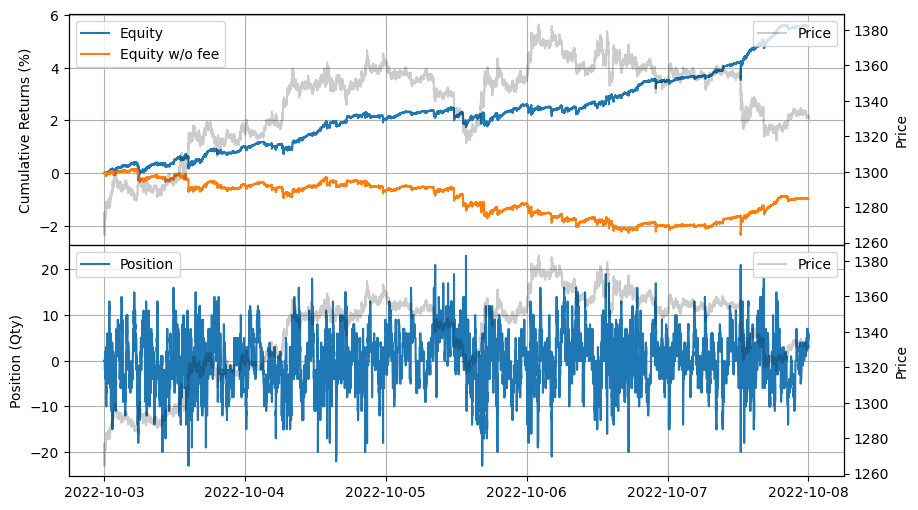
5日間のバックテストでは、クォートを継続的に投稿することで高い取引量を維持し、リベートを通じて利益を上げていることが明らかです。
[ ]:
asset = (
    BacktestAsset()
    .data(
        [
            "data/ethusdt_20221003.npz",
            "data/ethusdt_20221004.npz",
            "data/ethusdt_20221005.npz",
            "data/ethusdt_20221006.npz",
            "data/ethusdt_20221007.npz",
        ]
    )
    .initial_snapshot("data/ethusdt_20221002_eod.npz")
    .linear_asset(1.0)
    .intp_order_latency(
        [
            "latency/feed_latency_20221003.npz",
            "latency/feed_latency_20221004.npz",
            "latency/feed_latency_20221005.npz",
            "latency/feed_latency_20221006.npz",
            "latency/feed_latency_20221007.npz",
        ]
    )
    .power_prob_queue_model(2.0)
    .no_partial_fill_exchange()
    .trading_value_fee_model(-0.00005, 0.0007)
    .tick_size(0.01)
    .lot_size(0.001)
    .roi_lb(0.0)
    .roi_ub(3000.0)
    .last_trades_capacity(10000)
)

hbt = ROIVectorMarketDepthBacktest([asset])

recorder = Recorder(1, 5_000_000)

out = glft_market_maker(hbt, recorder.recorder)

hbt.close()

stats = LinearAssetRecord(recorder.get(0)).stats(book_size=30_000)
stats.summary()
| start | end | SR | Sortino | Return | MaxDrawdown | DailyNumberOfTrades | DailyTurnover | ReturnOverMDD | ReturnOverTrade | MaxPositionValue |
|---|---|---|---|---|---|---|---|---|---|---|
| datetime[μs] | datetime[μs] | f64 | f64 | f64 | f64 | f64 | f64 | f64 | f64 | f64 |
| 2022-10-03 00:00:00 | 2022-10-07 23:59:50 | 16.282366 | 20.682178 | 0.031145 | 0.009818 | 9463.81907 | 422.448163 | 3.172133 | 0.000015 | 34458.375 |
[25]:
stats.plot()
グリッドトレーディングの統合
Guéant–Lehalle–Fernandez-Tapia マーケットメイキングモデルから導出されたビッド価格とアスク価格からグリッドを作成します。
[ ]:
from numba import uint64
from numba.typed import Dict


@njit
def gridtrading_glft_mm(hbt, recorder):
    asset_no = 0
    tick_size = hbt.depth(asset_no).tick_size

    arrival_depth = np.full(10_000_000, np.nan, np.float64)
    mid_price_chg = np.full(10_000_000, np.nan, np.float64)

    t = 0
    prev_mid_price_tick = np.nan
    mid_price_tick = np.nan

    tmp = np.zeros(500, np.float64)
    ticks = np.arange(len(tmp)) + 0.5

    A = np.nan
    k = np.nan
    volatility = np.nan
    gamma = 0.05
    delta = 1
    adj1 = 1
    adj2 = 0.05

    order_qty = 1
    max_position = 20
    grid_num = 20

    # Checks every 100 milliseconds.
    while hbt.elapse(100_000_000) == 0:
        # --------------------------------------------------------
        # Records market order's arrival depth from the mid-price.
        if not np.isnan(mid_price_tick):
            depth = -np.inf
            for last_trade in hbt.last_trades(asset_no):
                trade_price_tick = last_trade.px / tick_size

                if last_trade.ev & BUY_EVENT == BUY_EVENT:
                    depth = np.nanmax([trade_price_tick - mid_price_tick, depth])
                else:
                    depth = np.nanmax([mid_price_tick - trade_price_tick, depth])
            arrival_depth[t] = depth

        hbt.clear_last_trades(asset_no)
        hbt.clear_inactive_orders(asset_no)

        depth = hbt.depth(asset_no)
        position = hbt.position(asset_no)
        orders = hbt.orders(asset_no)

        best_bid_tick = depth.best_bid_tick
        best_ask_tick = depth.best_ask_tick

        prev_mid_price_tick = mid_price_tick
        mid_price_tick = (best_bid_tick + best_ask_tick) / 2.0

        # Records the mid-price change for volatility calculation.
        mid_price_chg[t] = mid_price_tick - prev_mid_price_tick

        # --------------------------------------------------------
        # Calibrates A, k and calculates the market volatility.

        # Updates A, k, and the volatility every 5-sec.
        if t % 50 == 0:
            # Window size is 10-minute.
            if t >= 6_000 - 1:
                # Calibrates A, k
                tmp[:] = 0
                lambda_ = measure_trading_intensity(
                    arrival_depth[t + 1 - 6_000 : t + 1], tmp
                )
                if len(lambda_) > 2:
                    lambda_ = lambda_[:70] / 600
                    x = ticks[: len(lambda_)]
                    y = np.log(lambda_)
                    k_, logA = linear_regression(x, y)
                    A = np.exp(logA)
                    k = -k_

                # Updates the volatility.
                volatility = np.nanstd(mid_price_chg[t + 1 - 6_000 : t + 1]) * np.sqrt(
                    10
                )

        # --------------------------------------------------------
        # Computes bid price and ask price.

        c1, c2 = compute_coeff(gamma, gamma, delta, A, k)

        half_spread_tick = (c1 + delta / 2 * c2 * volatility) * adj1
        skew = c2 * volatility * adj2

        reservation_price_tick = mid_price_tick - skew * position

        bid_price_tick = np.minimum(
            np.round(reservation_price_tick - half_spread_tick), best_bid_tick
        )
        ask_price_tick = np.maximum(
            np.round(reservation_price_tick + half_spread_tick), best_ask_tick
        )

        bid_price = bid_price_tick * tick_size
        ask_price = ask_price_tick * tick_size

        grid_interval = max(np.round(half_spread_tick) * tick_size, tick_size)

        bid_price = np.floor(bid_price / grid_interval) * grid_interval
        ask_price = np.ceil(ask_price / grid_interval) * grid_interval

        # --------------------------------------------------------
        # Updates quotes.

        # Creates a new grid for buy orders.
        new_bid_orders = Dict.empty(np.uint64, np.float64)
        if position < max_position and np.isfinite(bid_price):
            for i in range(grid_num):
                bid_price_tick = round(bid_price / tick_size)

                # order price in tick is used as order id.
                new_bid_orders[uint64(bid_price_tick)] = bid_price

                bid_price -= grid_interval

        # Creates a new grid for sell orders.
        new_ask_orders = Dict.empty(np.uint64, np.float64)
        if position > -max_position and np.isfinite(ask_price):
            for i in range(grid_num):
                ask_price_tick = round(ask_price / tick_size)

                # order price in tick is used as order id.
                new_ask_orders[uint64(ask_price_tick)] = ask_price

                ask_price += grid_interval

        order_values = orders.values()
        while order_values.has_next():
            order = order_values.get()
            # Cancels if a working order is not in the new grid.
            if order.cancellable:
                if (order.side == BUY and order.order_id not in new_bid_orders) or (
                    order.side == SELL and order.order_id not in new_ask_orders
                ):
                    hbt.cancel(asset_no, order.order_id, False)

        for order_id, order_price in new_bid_orders.items():
            # Posts a new buy order if there is no working order at the price on the new grid.
            if order_id not in orders:
                hbt.submit_buy_order(
                    asset_no, order_id, order_price, order_qty, GTX, LIMIT, False
                )

        for order_id, order_price in new_ask_orders.items():
            # Posts a new sell order if there is no working order at the price on the new grid.
            if order_id not in orders:
                hbt.submit_sell_order(
                    asset_no, order_id, order_price, order_qty, GTX, LIMIT, False
                )

        # --------------------------------------------------------
        # Records variables and stats for analysis.

        t += 1

        if t >= len(arrival_depth) or t >= len(mid_price_chg):
            raise Exception

        # Records the current state for stat calculation.
        recorder.record(hbt)
    return out[:t]
[ ]:
asset = (
    BacktestAsset()
    .data(
        [
            "data/ethusdt_20221003.npz",
            "data/ethusdt_20221004.npz",
            "data/ethusdt_20221005.npz",
            "data/ethusdt_20221006.npz",
            "data/ethusdt_20221007.npz",
        ]
    )
    .initial_snapshot("data/ethusdt_20221002_eod.npz")
    .linear_asset(1.0)
    .intp_order_latency(
        [
            "latency/feed_latency_20221003.npz",
            "latency/feed_latency_20221004.npz",
            "latency/feed_latency_20221005.npz",
            "latency/feed_latency_20221006.npz",
            "latency/feed_latency_20221007.npz",
        ]
    )
    .power_prob_queue_model(2.0)
    .no_partial_fill_exchange()
    .trading_value_fee_model(-0.00005, 0.0007)
    .tick_size(0.01)
    .lot_size(0.001)
    .roi_lb(0.0)
    .roi_ub(3000.0)
    .last_trades_capacity(10000)
)

hbt = ROIVectorMarketDepthBacktest([asset])

recorder = Recorder(1, 5_000_000)

out = gridtrading_glft_mm(hbt, recorder.recorder)

hbt.close()

stats = LinearAssetRecord(recorder.get(0)).stats(book_size=30_000)
stats.summary()
| start | end | SR | Sortino | Return | MaxDrawdown | DailyNumberOfTrades | DailyTurnover | ReturnOverMDD | ReturnOverTrade | MaxPositionValue |
|---|---|---|---|---|---|---|---|---|---|---|
| datetime[μs] | datetime[μs] | f64 | f64 | f64 | f64 | f64 | f64 | f64 | f64 | f64 |
| 2022-10-03 00:00:00 | 2022-10-07 23:59:50 | 19.774661 | 24.630456 | 0.055856 | 0.007438 | 5878.736082 | 262.524795 | 7.509437 | 0.000043 | 30859.215 |
[28]:
stats.plot()
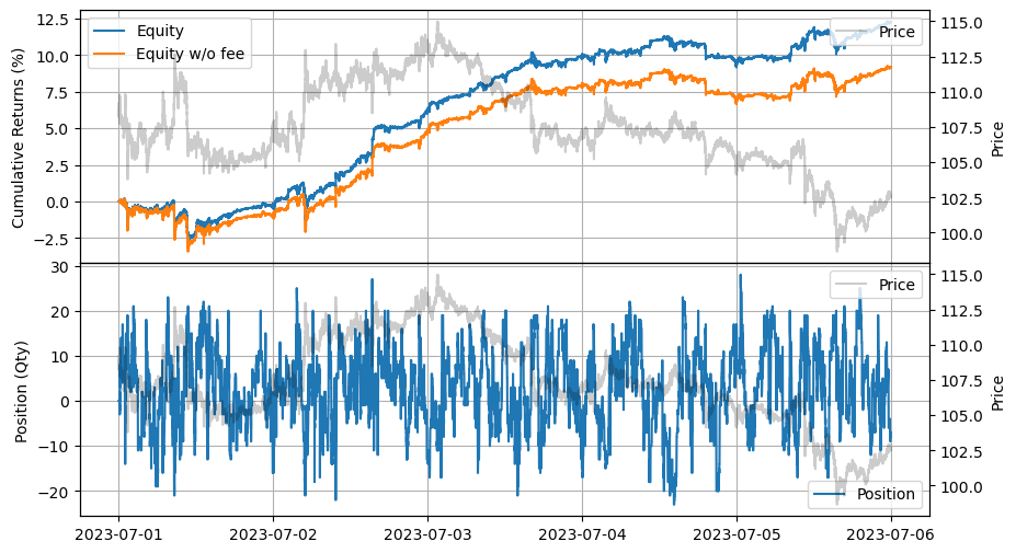
他のコインでもうまく機能することがわかります。次の例では、複数の市場を作成してリスク調整後のリターンを向上させる方法を示します。
[ ]:
asset = (
    BacktestAsset()
    .data(
        [
            "data/ltcusdt_20230701.npz",
            "data/ltcusdt_20230702.npz",
            "data/ltcusdt_20230703.npz",
            "data/ltcusdt_20230704.npz",
            "data/ltcusdt_20230705.npz",
        ]
    )
    .initial_snapshot("data/ltcusdt_20230630_eod.npz")
    .linear_asset(1.0)
    .intp_order_latency(
        [
            "latency/feed_latency_20230701.npz",
            "latency/feed_latency_20230702.npz",
            "latency/feed_latency_20230703.npz",
            "latency/feed_latency_20230704.npz",
            "latency/feed_latency_20230705.npz",
        ]
    )
    .power_prob_queue_model(2.0)
    .no_partial_fill_exchange()
    .trading_value_fee_model(-0.00005, 0.0007)
    .tick_size(0.01)
    .lot_size(0.001)
    .roi_lb(0.0)
    .roi_ub(300.0)
    .last_trades_capacity(10000)
)

hbt = ROIVectorMarketDepthBacktest([asset])

recorder = Recorder(1, 5_000_000)

out = gridtrading_glft_mm(hbt, recorder.recorder)

hbt.close()

stats = LinearAssetRecord(recorder.get(0)).stats(book_size=3000)
stats.summary()
| start | end | SR | Sortino | Return | MaxDrawdown | DailyNumberOfTrades | DailyTurnover | ReturnOverMDD | ReturnOverTrade | MaxPositionValue |
|---|---|---|---|---|---|---|---|---|---|---|
| datetime[μs] | datetime[μs] | f64 | f64 | f64 | f64 | f64 | f64 | f64 | f64 | f64 |
| 2023-07-01 00:00:00 | 2023-07-05 23:59:50 | 17.17992 | 23.062973 | 0.122535 | 0.032973 | 3425.879303 | 122.800909 | 3.716196 | 0.0002 | 2930.06 |
[30]:
stats.plot()
まとめ
これまでに、モデルを実際の例に適用する方法を示しました。
より効果的なマーケットメイキングアルゴリズムを考える際には、このモデルを次のカテゴリに分けて検討してください:
ハーフスプレッド: ハーフスプレッドは取引強度と市場のボラティリティの関数です。取引強度に対して指数関数を使用することは、全範囲に対して適切ではないかもしれません。取引強度をハーフスプレッドに変換するためのより洗練されたアプローチを開発することができます。さらに、ここでは過去の取引強度と市場のボラティリティを使用していますが、短期的な取引強度とボラティリティを予測して、市場の状況の変化に迅速に対応することができます。これには、ニュース、イベント、流動性の真空などを使用してボラティリティの爆発を予測する戦略が含まれるかもしれません。
スキュー: スキューも取引強度と市場のボラティリティの関数です。このモデルでは在庫リスクのみが考慮されていますが、複数の市場を作成する際には他のリスクも考慮することができます。BARRAは他のリスクを同様に管理する良い例です。
公正価格の設定: このモデルでは公正価格がミッドプライスと等しいとされていますが、マイクロプライスや関連資産を通じた公正価格の設定などの予測を組み込むことで、戦略を強化することができます。
ヘッジ: 複数の市場を作成する際には、ヘッジはリスク管理のための貴重なツールです。
今後の例では、いくつかのトピックについてさらに詳しく説明します。